Thesis: Using Individual-level Models to Model Spatio-temporal Combustion Dynamics. Supervisors: Rob Deardon and Zeng Feng (co-author Dr. John Braun). This involved modelling the spatio-temporal combustion dynamics of fire in a Bayesian framework
University of Guelph, PhD (Applied Statistics)
Thesis: Non-Elliptical and Fractionally-Supervised Classification. Supervisor: Paul D. McNicholas. This involved model-based classification with a particular emphasis on non-elliptical distributions.
Post (post?) Graduate Education
Postdoctoral Fellow at McGill University
Under the supervision of Dr. David Stephens, this work focused on the statistical and computational challenges associated with analyzing genetic data. It involved clustering and modeling HIV DNA sequences.
Postdoctoral Fellow at UBCO
Awarded by NSERC (Natural Sciences and Engineering Research Council of Canada), this research involved collaborations with faculty from several disciplines (eg. Medical Physics, Biology, and Chemistry) and was supervised by Dr. Jason Loeppky.
Instructor at UBCO
A three-year contract position in the Department of Computer Science, Mathematics, Physics, and Statistics.
Courses I have taught at UBCO
Stat 230: Introductory Statistics DATA 101: Making Predictions with Data DATA 301: Introduction to Data Analytics DATA 311: Machine Learning DATA 543: Data Collection DATA 550: Data Visualization DATA 570: Predictive Modelling DATA 582: Bayesian Inference DATA 599: Capstone
Research Interests
- apply my statistical background in the pedagogical domain
- enhance student learning and promote statistical literacy
- make Data Science approachable
Past:
- models for fire dynamics
- unsupervised learning
- supervised learning
- semi-supervised learning
- robust mixture-models - models for infectious disease
Future:
- learning analytics
- curriculum development
- tools for teaching
- contributions to the body of teaching, learning, and technology
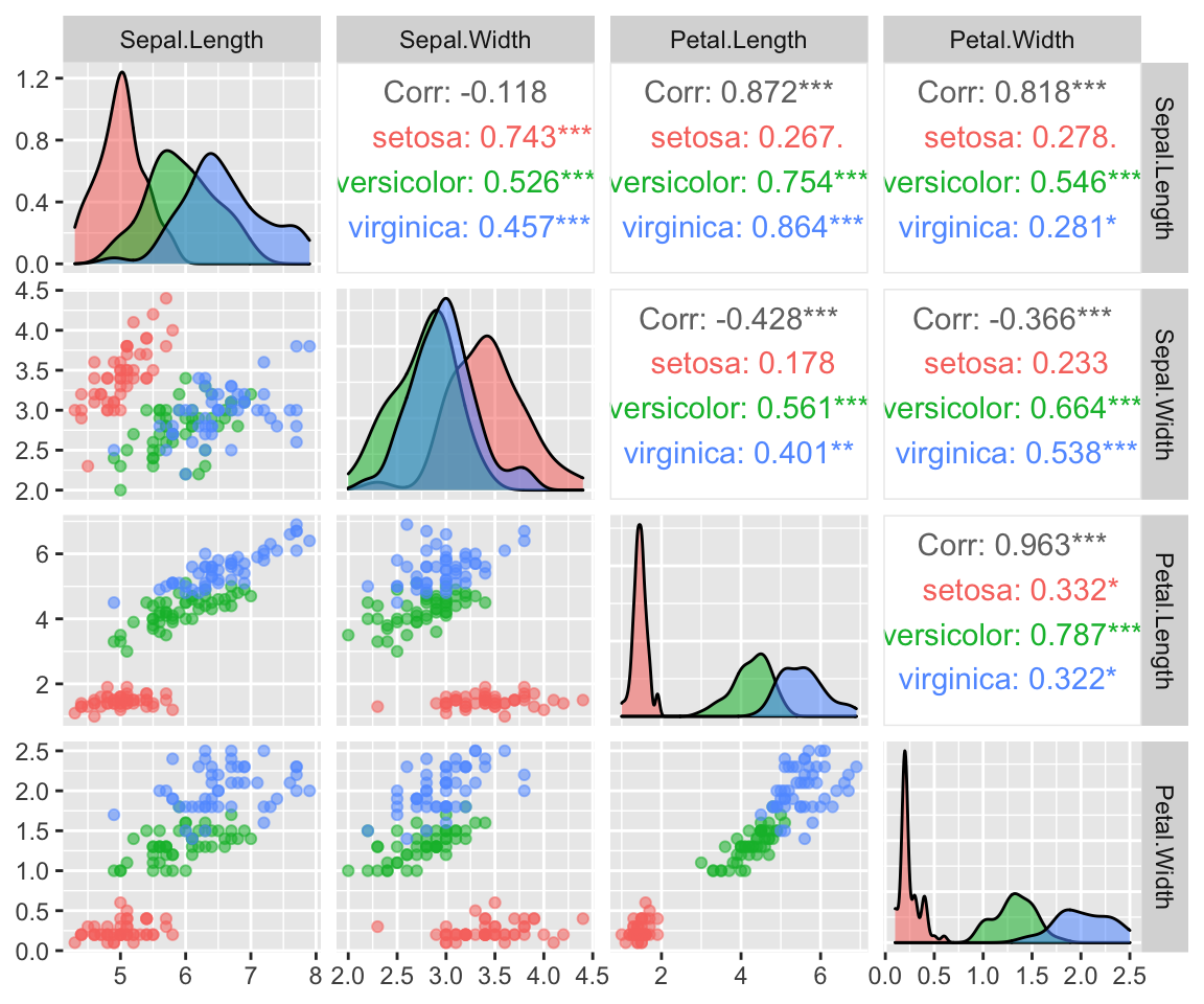
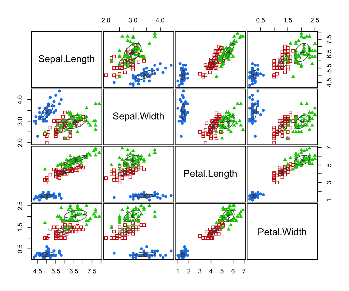
Here i am using “clusters” as groups of data that clump together, but really these are just know classifcation corresponding to the species are Iris setosa, versicolor, and virginica.
We can see that these species form distinct clusters (esp in the Sepal.Width vs Petal.Width scatterplot)
library(ggplot2)# install.packages("GGally")library(GGally)ggpairs(iris, # Data framecolumns =1:4, # Columnsaes(color = Species, # Color by group (cat. variable)alpha =0.5)) # Transparency
The goal of clustering1 (a form of unsupervised learning) is to find groups such that all observations are
more similar to observations inside their group and
more dissimilar to observations in other groups.
Cluster analysis is widely adopted by various applications like image processing, neuroscience, economics, network communication, medicine, recommendation systems, customer segmentation, to name a few.
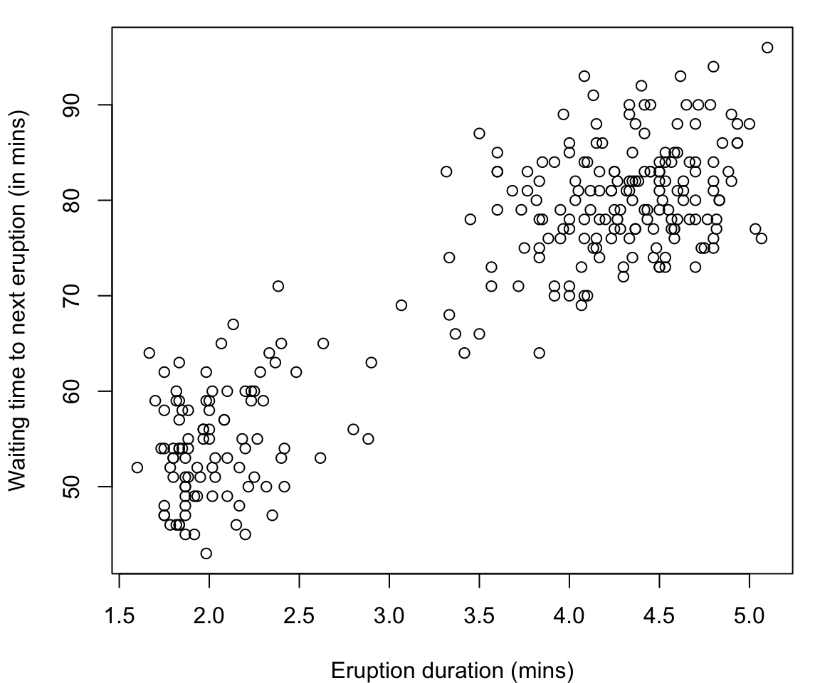
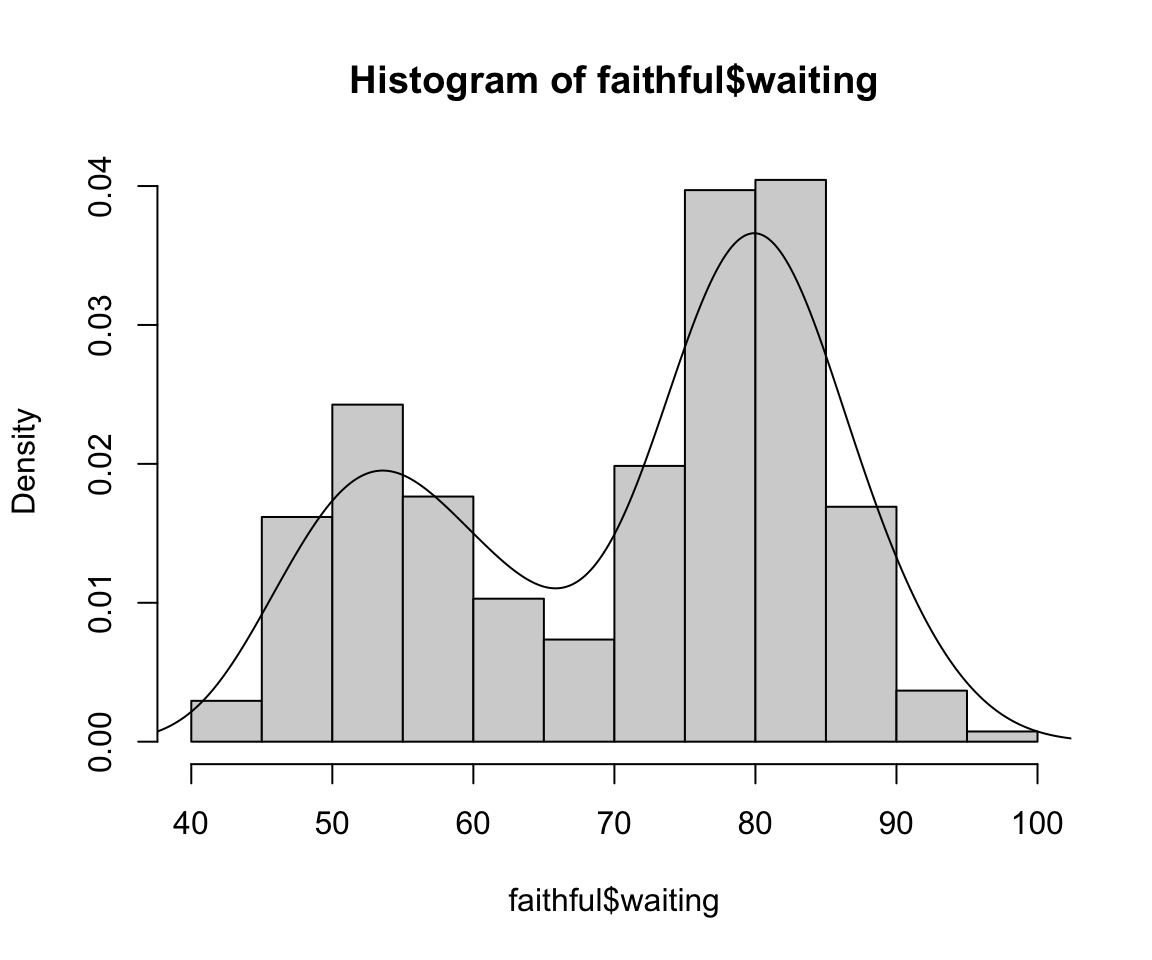
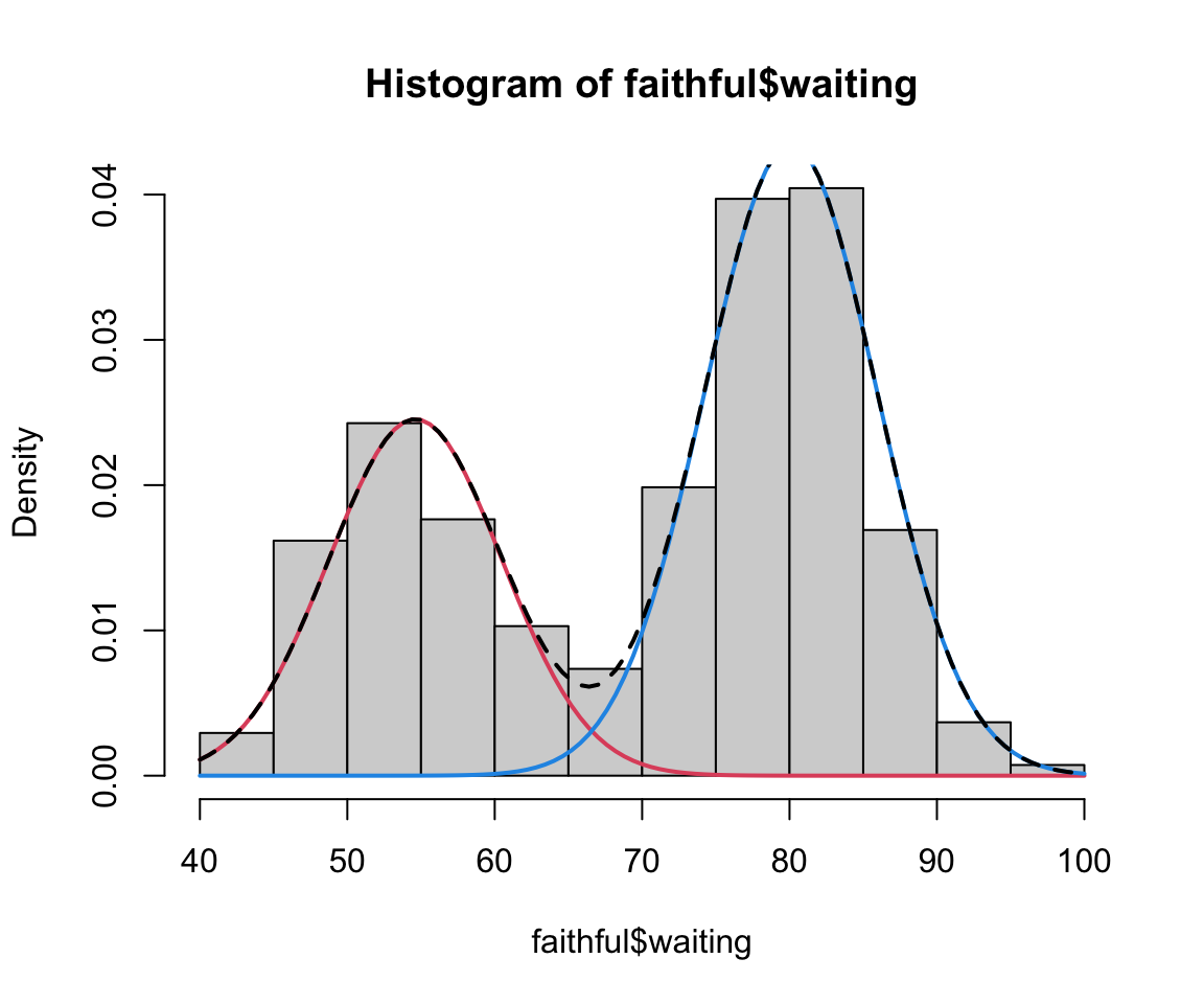
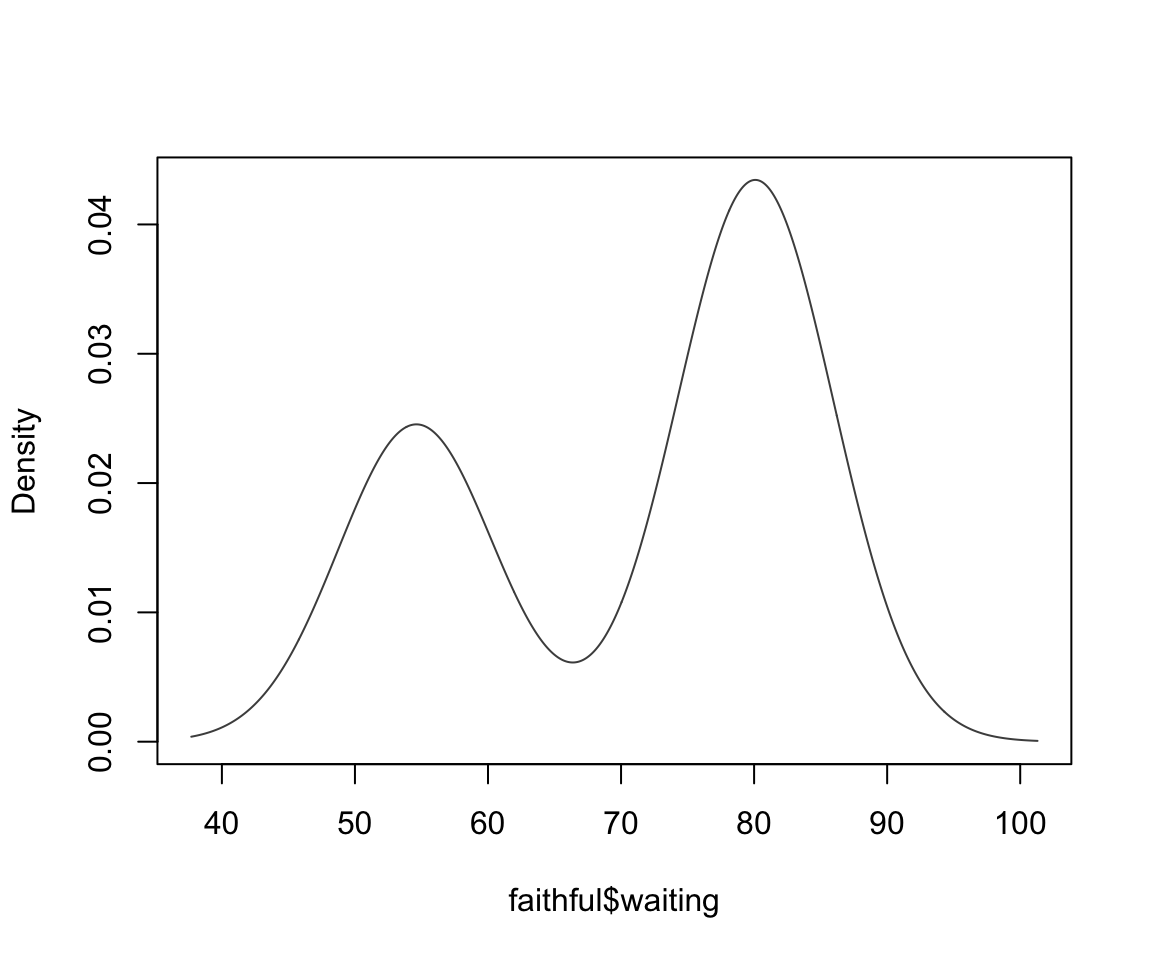
The faithful dataset in R contains the measurements on time to eruption, and length of eruption time of the Old Faithful geyser in Yellowstone National Park.
The data frame consists of 272 observations on 2 variables:
eruptions Eruption time in mins (numeric)
waiting Waiting time to next eruption in mins (numeric)
N.B. to see the help file for any dataset (or function in R) use ?name_of_thing
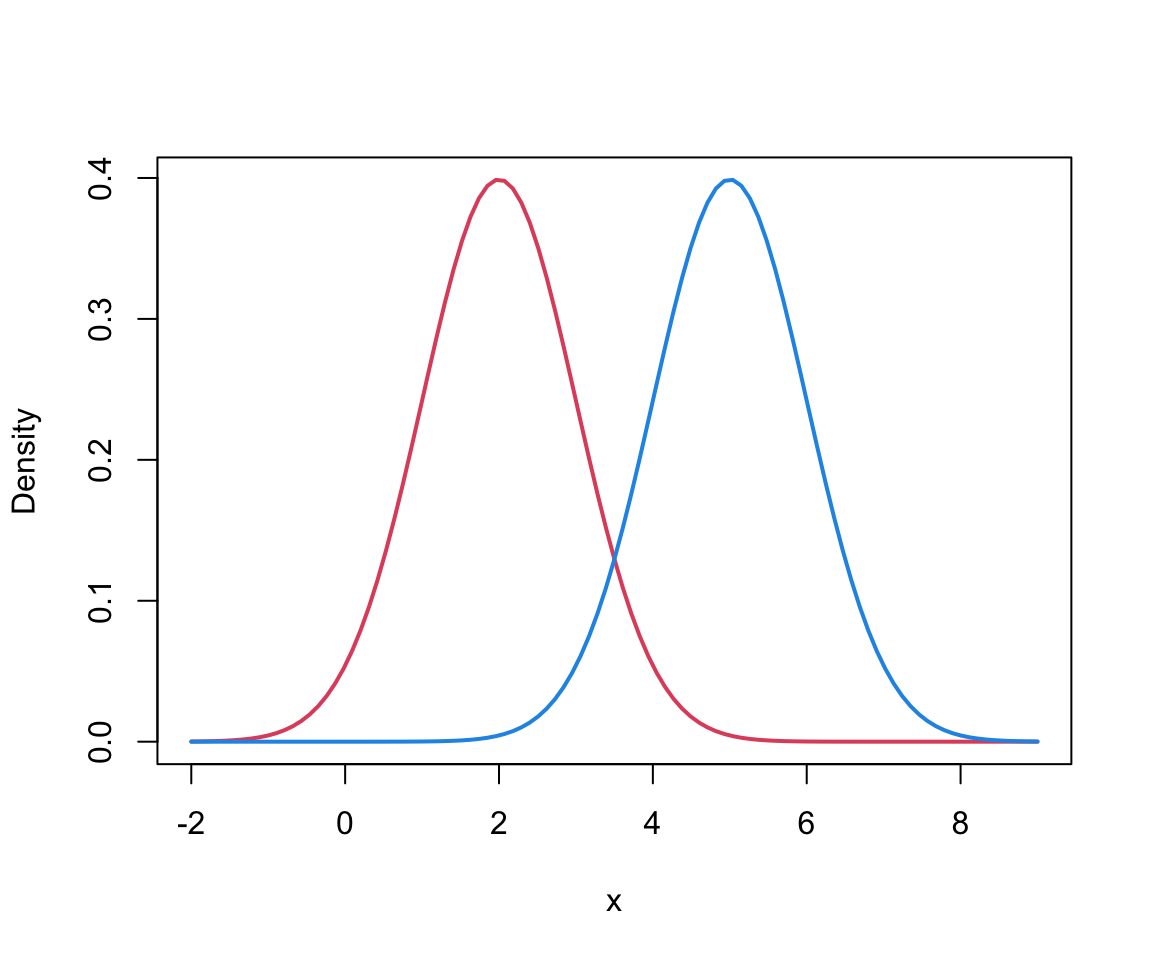
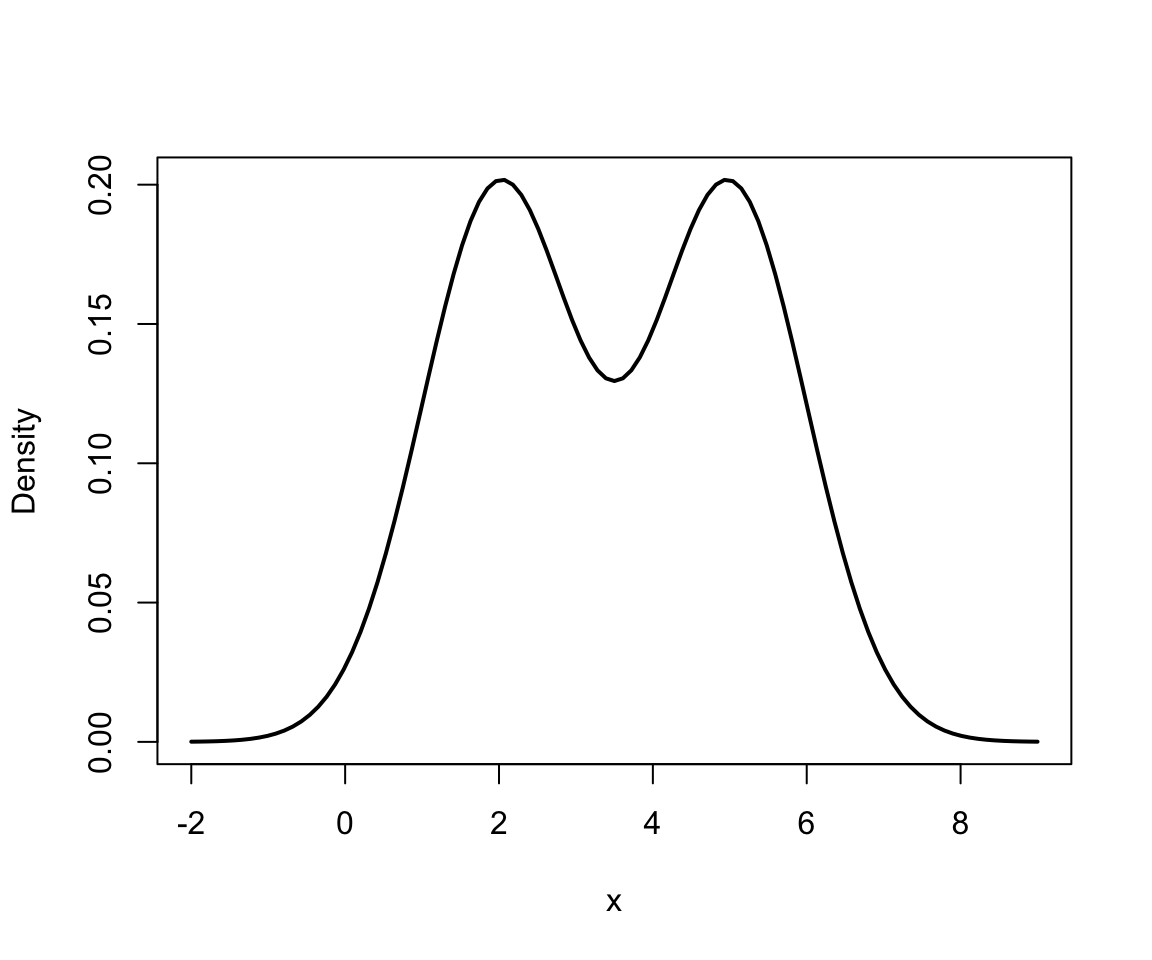
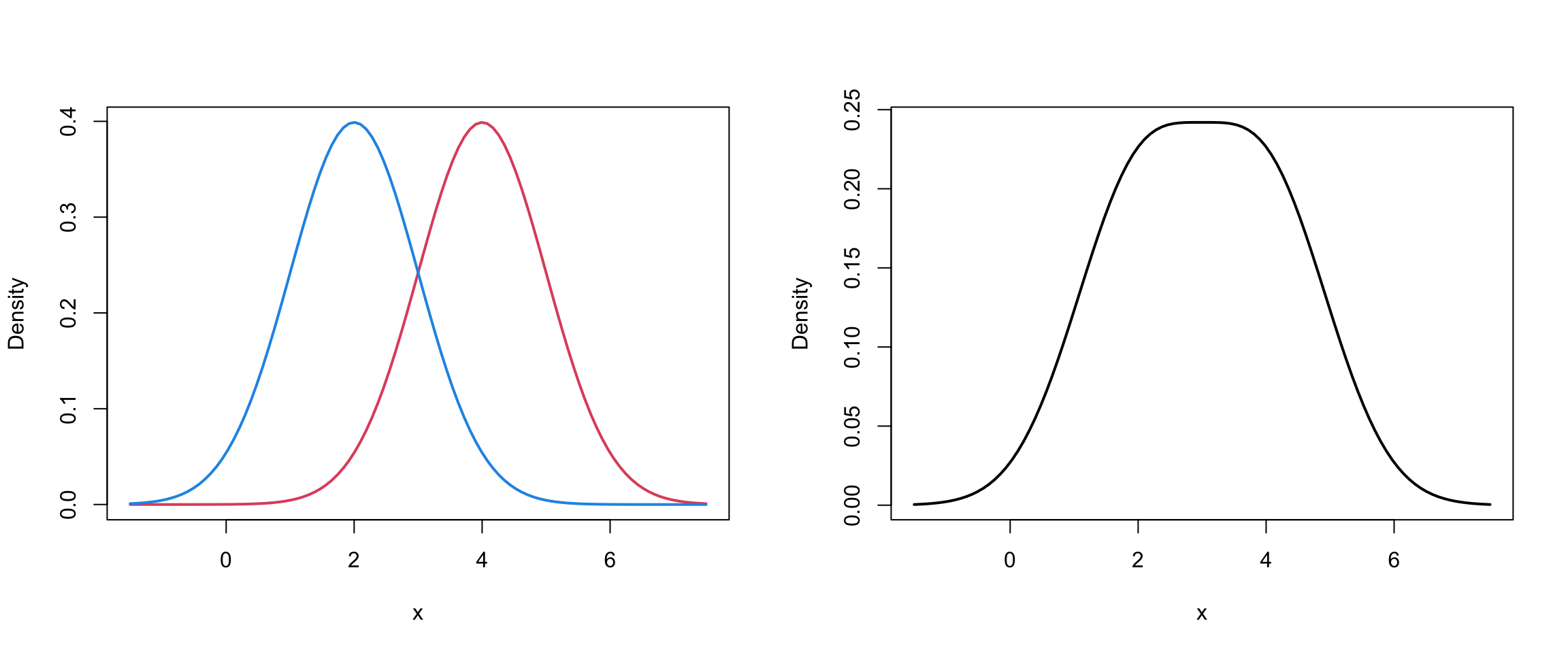
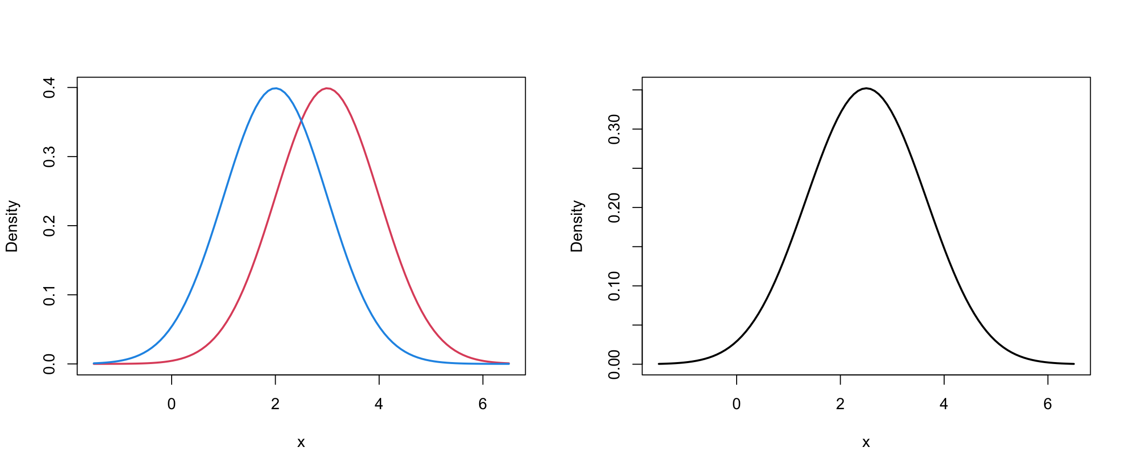
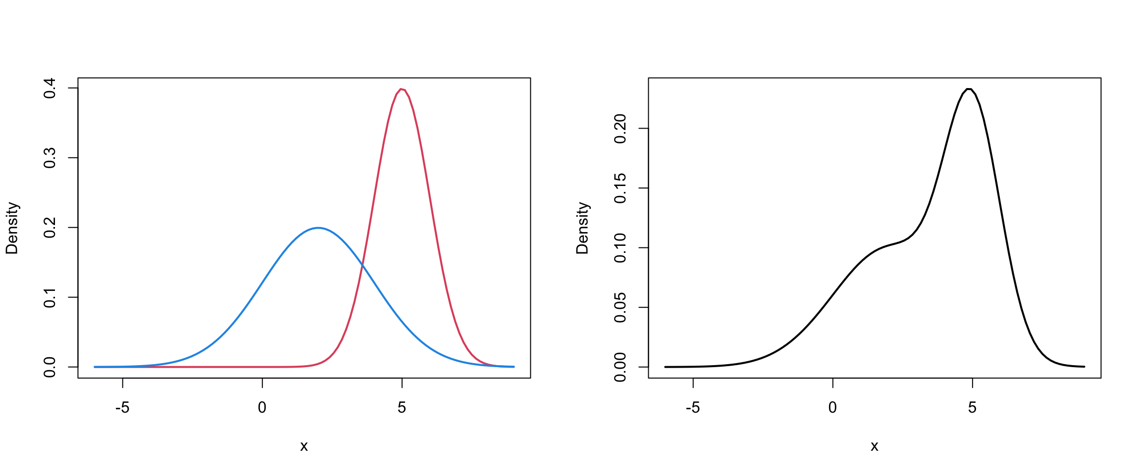
Mixture models are just a convex combination of statistical distributions. In general, for a random vector \(\mathbf{X}\), a mixture distribution is defined by \[f(\mathbf{x}) = \sum_{g=1}^G \pi_g p_g(\mathbf{x} \mid \theta_g)\] where \(G\) is the number of groups, \(0 \leq \pi_g \leq 1\) and \(\sum_{g=1}^G \pi_g = 1\) and \(p_g(\mathbf{x} \mid \theta_g)\) are statistical distributions with parameters \(\theta_g\).
Terminology
The \(\pi_g\) are called mixing proportions and we will write \(\bf{\pi} = (\pi_1, \pi_2, \dots, \pi_G)\)
The \(p_g(\mathbf{x})\) are called component densities
Since the \(p_g(\mathbf{x})\) are densities, \(f(\mathbf{x})\) describes a density called a \(g\)-component finite mixture density.
Statistical Distributions
In theory, \(p_g(\mathbf{x} \mid \theta_g)\) could be a different distribution type for each \(g\).
In practice, however, \(p_g(\mathbf{x} \mid \theta_g)\) is assumed to be the same across groups, but with different \(\theta_g\).
Most commonly, we assume a a Gaussian mixture model (GMM) where \(p_g(\mathbf{x} \mid \theta_g)\) is assumed to be multivariate Gaussian (aka multivariate Normal), denoted \(\phi(\mathbf{x} | \mu_g, \mathbf{\Sigma}_g)\)
Gaussian Mixture model
Thus \(f(\mathbf{x})\) — sometimes written \(f(\mathbf{x} | \Theta)\) or \(f(\mathbf{x} ; \Theta)\) — is a Gaussian mixture model would have the form: \[\begin{align}
f(\mathbf{x} | \Theta) &= \sum_{g=1}^G \pi_g \phi(\mathbf{x} \mid \boldsymbol\mu_g, \mathbf{\Sigma}_g) \\
&= \sum_{g=1}^G \pi_g \frac{|\mathbf{\Sigma}|^{-1/2}}{(2\pi)^{k/2}} \exp
\left(
- \frac{1}{2}
(\mathbf{x} - \boldsymbol{\mu}_g)^{\mathrm {T}}
\mathbf{\Sigma}^{-1}
(\mathbf{x} - \boldsymbol{\mu}_g)
\right)
\end{align}\] where \(\phi\) denote the normal distribution, \(\boldsymbol{\mu}_g\) is the mean vector for group \(g\) and \(\mathbf{\Sigma}_g\) is the covariance matrix for group \(g\), and \(\Theta = \{\boldsymbol{\mu}_1, ..., \boldsymbol{\mu}_G, \mathbf{\Sigma}_1, ..., \mathbf{\Sigma}_G, \pi_1, ..., \pi_G\}\)
Distribution Alternatives
Other robust alternatives include:
Mixtures of Student-\(t\) distributions1 (heavier tails)
'densityMclust' model object: (E,2)

Available components:
 [1] "call"           "data"           "modelName"      "n"
 [5] "d"              "G"              "BIC"            "loglik"
 [9] "df"             "bic"            "icl"            "hypvol"
[13] "parameters"     "z"              "classification" "uncertainty"
[17] "density"
Identifiability I
Inference for finite mixture modles is typical in that we want to estimate parameters \(\Theta = \{\theta_1, ... , \theta_G, \pi_1, ...,\pi_G\}\)
However, this estimation is only meaningful if \(\Theta\) is identifiable.
In general, a family of densities \(\{ p(\mathbf{x} | \Theta) : \Theta \in \Omega \}\) is identifiable if: \[p(\mathbf{x} | \Theta) = p(\mathbf{x} |\Theta^*) \iff \Theta^* = \Theta\] In the case of mixture models this gets a bit complicated…
Identifiability II
One problem is that component labels may be permuted:
The identifiable condition is not satisfied because the component labels can be interchanged yet \(p(x | \Theta) = p(x | \Theta^*)\)
As [MG] point out, even though this class of mixtures may be identifiable, \(\Theta\) is not.
Identifiability III
The identifiability issue that arises due to the interchanging of component labels can be handled by imposing appropriate constraints on \(\Theta\)
For example, the \(\pi_g\) could be constrained so that \(\pi_i \geq \pi_k\) for \(i>k\).
Also we can avoid empty components by insisting that \(\pi_g > 0\) for all \(g\).
Mixture Models for clustering
Finite mixture models are ideally suited for clustering
Clusters correspond to the \(1,...,g,...G\) sub-populations/groups/components in a finite mixtures model.
So, let’s attempt the to derive the MLE of the Gaussian mixture model …
The Likelihood
The likelihood function for this mixture is \[\begin{align}
L(\Theta) &= f(\mathbf{x} | \Theta) = \Pi_i \left[ \sum_{g=1}^G \pi_g \phi(\mathbf{x} \mid \boldsymbol\mu_g, \mathbf{\Sigma}_g) \right]
\end{align}\] and the so-called log-likelihood is: \[\begin{align}
\ell(\Theta) &= \log(L(\Theta)) = \sum_{i=1}^N \log\left[ \sum_{g=1}^G \pi_g \phi(\mathbf{x} \mid \boldsymbol\mu_g, \mathbf{\Sigma}_g) \right]
\end{align}\]
If you try to differentiate w.r.t. to \(\mu_g\), set =0, and solve, you would find that this has no analytic solution
EM algorithm
Most commonly, we use the expectation-maximization (EM) algorithm, which helps us find parameter estimates with missing data (group memberships are missing).
More generally, the EM is an iterative algorithm for finding maximum likelihood parameters in statistical models, where the model depends on unobserved latent variables.
We assume that each observed data point has a corresponding unobserved latent variable specifying the mixture component to which each data point belongs.
Latent Variable
We introduce a new latent1 variable that represents the group memberships: \[\begin{equation}
Z_{ig} = \begin{cases}
1 & \text{if } \mathbf{x}_i \text{ belongs to group }g \\
0 & \text{otherwise}
\end{cases}
\end{equation}\]
We call \(\{X, Z\}\) our “complete” data.
Now that we have that, let’s look at a non-technical summary of the EM algorithm…
Latent Variable Representation
We can now represent our mixture model \[\begin{align}
f({x} | \Theta) &= \sum_{g=1}^G \pi_g \phi(\mathbf{x} \mid \boldsymbol\mu_g, \mathbf{\Sigma}_g) \\
&= \sum_{g=1}^G p(Z_{ig} = 1) p(x \mid Z_{ig} = 1)
\end{align}\] This is sometimes called the latent variable representation of the mixture model.
Complete Likelihood
The “complete” likelihood takes the form: \[\begin{equation}
L_c(\Theta) = \prod_{i=1}^n \prod_{g=1}^G \pi_g^{\hat{z}_{ig}} \phi(x_i|\mu_g, \sigma_g)^{\hat{z}_{ig}}
\end{equation}\] so the complete log-likelihood, \(\log \left( L_c(\Theta) \right)\), takes the form: \[\begin{align}
\ell_c(\Theta) &= \sum_{i=1}^n \sum_{g=1}^G \hat{z}_{ig} \left[ \log (\pi_g) + \log (\phi(x_i|\mu_g, \sigma_g) )\right]
\end{align}\]
We’ll work with univariate normal distribution for simplicity.
EM Pseudocode
Start the algorithm with random values for \(\hat z_{ig}\).
Mstep: Assuming those \(\hat{z}_{ig}\) are correct, find the maximum likelihood estimates (MLE) of \(\boldsymbol{\mu}_g\) and \(\mathbf{\Sigma}_g\)
Estep: Assuming those parameters are correct, find the expected value of group memberships \[\hat{z}_{ig} = \frac{\pi_g \phi(\mathbf{x} \mid \boldsymbol{\mu}_g, \mathbf{\Sigma}_g) }{\sum_{g=1}^G \pi_g \phi(\mathbf{x} \mid \boldsymbol{\mu}_g, \mathbf{\Sigma}_g)}\]
Repeat 2. and 3. until “changes” are minimal.
Estep
For the “E-step”, i.e. expectation step …
Mstep
For the “M-step”, i.e. maximization step …
Fuzzy z’s
The resulting \(\hat{z}_{ig}\) are not going to be 0’s and 1’s when the algorithm converges.
For each observation \(\mathbf{x}_i\) we end up with vector of probabilities (\(\hat{z}_{i1}\),…,\(\hat{z}_{iG}\)) which we denote by \(\hat{\mathbf{z}}_i\)
So, for example, observation \(\mathbf{x}_i\) might have a corresponding estimate of \(\hat{\mathbf{z}}_i = (0.25, 0.60, 0.15)\)–> in this case\(\mathbf{x}_i\) would get assigned to group 2
But! We usually still want a “best” guess as to which group the observation belongs to. Continuing with example above what do you think might happen …
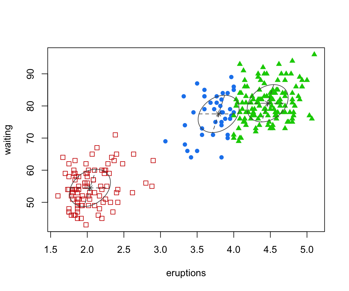
MCLUST example
To see this in action, lets take a closer look at the MCLUST output when it was fit to our old faithful geyser data.
One solution to problem 1 is is start your algorithm and several different initialization
Another potential solution it to start in a smart location (to be determined by some other clustering method, eg. kmeans)
Problem 2
The total number of “free” parameters in a GMM is: \[\begin{equation}
(G-1) + Gp + Gp(p+1)/2
\end{equation}\]
\(Gp(p+1)/2\) of these are from the group covariance matrices \(\mathbf{\Sigma}_1,..., \mathbf{\Sigma}_G\)
For the EM, we have to invert these \(G\) covariance matrices for each iteration of the algorithm.
This can get quite computationally expensive…
Common Covariance
One potential solution to problem 2 is to assumes that the covariance are equal across groups
The constraint of \(\mathbf{\Sigma}_g = \mathbf{\Sigma}\) for all \(g\) this reduces to \(p(p+1)/2\) free parameters in the common covariance matrix.
This however is a very strong assumption about the underlying data, so perhaps we could impose a softer constraint …
Towards MCLUST
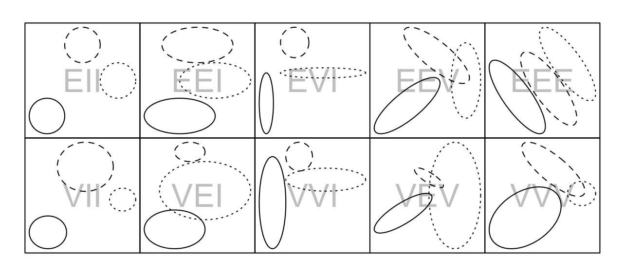
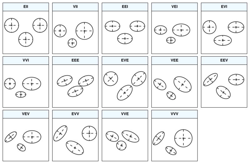
MCLUST exploits an eigenvalue decomposition of the group covariance matrices to give a wide range of structures that uses between 1 and \(Gp(p+1)/2\) free parameters.
The eigenvalue decomposition has the form \[\begin{equation}
\mathbf{\Sigma}_g = \lambda_g \mathbf{D}_g \mathbf{A}_g \mathbf{D}'_g
\end{equation}\] where \(\lambda_g\) is a constant, \(\mathbf{D}_g\) is a matrix consisting of the eigenvectors of \(\mathbf{\Sigma}_g\) and \(\mathbf{A}_g\) is a diagonal matrix with entries proppotional the the eigenvalues of \(\mathbf{\Sigma}_g\).
Constraints & MCLUST
We may constrain the components of the eigenvalue decomposition of \(\mathbf{\Sigma}_g\) across groups of the mixture model
Furthermore, the matrices \(\mathbf{D}_g\) and \(\mathbf{A}_g\) may be set to the identity matrix \(\mathbf{I}\)
Fraley & Ratery (2000) describe the mclust software, which is available as an R package that efficiently performs this constrained model-based clustering.
MCLUST models
Notes: E = equal; S=spherical; V=variable; AA=axis-aligned
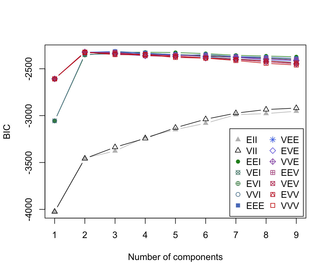
By default, MCLUST will fit a g-component mixture model for all 14 models models for \(g\) = 1, 2, … 9.
For each of these 126 models, a BIC value is calculated.
The BIC
The Bayesian Information Criterion or BIC (Schwarz, 1978) is one of the most widely known and used tools in statistical model selection. The BIC can be written: \[\begin{equation}
\text{BIC} = 2 \ell(x, \hat \theta) - \rho \log{N}
\end{equation}\] where \(\ell\) is the log-likelihood, \(\hat{\theta}\) is the MLE of \(\theta\), \(\rho\) is the # of free parameters and \(N\) is the # of observations.
It can be shown that the BIC gives consistent estimates of the number of components in a mixtures model under certain regulator conditions (Keribin, 1988 , 2000)
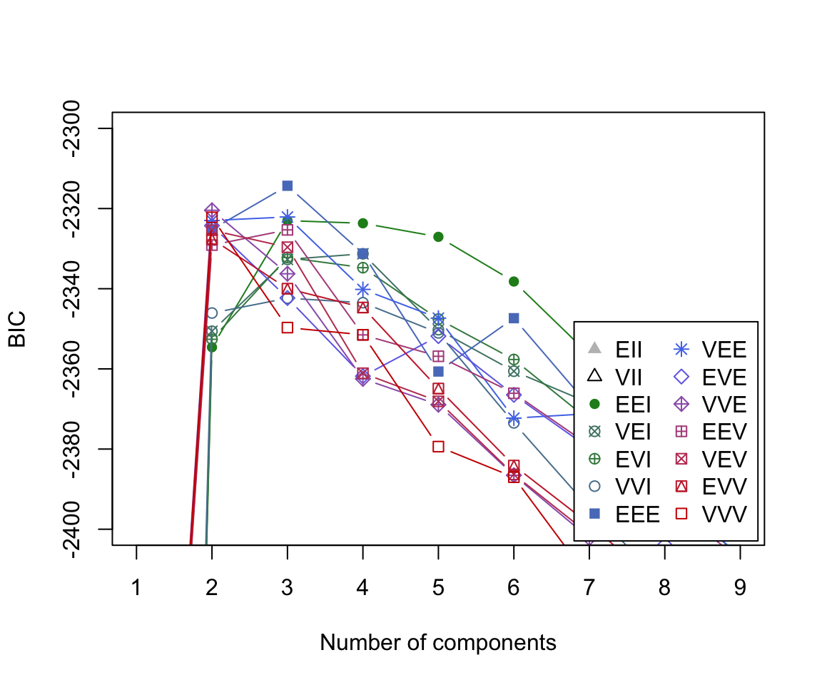
BIC plot (zoomed)
plot(mod2$BIC, ylim=c(-2400, -2300))
The BIC plot reveals that the model which obtains the largest BIC value is the 3-component mixture model with the ‘EEE’ covariance structure.
Pros
Why Mixture Model-based Clustering?
Mathematically and statistically sound using standard theory
Parameter estimation is built-in, along with number of clusters via model selection
Provides a probabilistic answer to the question “does observation \(i\) belong to group \(G\)?”
Adaptable, eg. data with outliers/skewness can be handled by non-Gaussian densities
Cons
Cons (a.k.a. open avenues for research)
Computationally intensive (takes time to estimate and invert covariance matrices; not feasible for small \(n\) large \(p\) without some decomposition)
Model-selection method is still viewed as an open problem by many practitioners — BIC grudgingly accepted
Traditional parameter estimation via EM algorithm prone to local maxima, overconfidence in clustering probabilities, and several other issues
Comments
Before we jump into the specifics, it is important to realize that there are many different clustering algorithms used in data science. For example:
We will be focusing on the mixture modeling paradigm …