Data 311: Machine Learning
Lecture 5: Multiple linear regression II
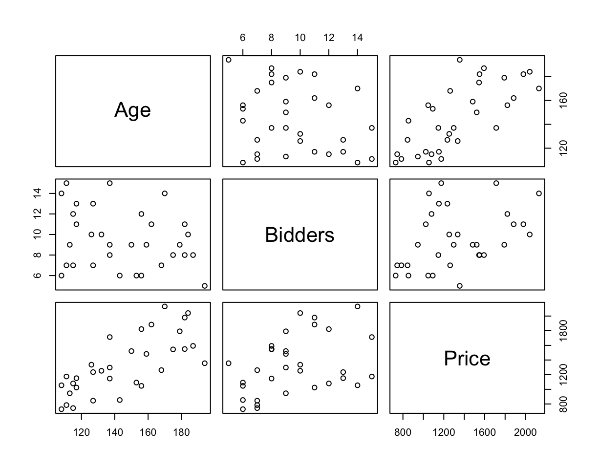
Example: Clock Auction

The data give the selling price,
Priceat auction of 32 antique grandfather clocks.Also recorded is the age of the clock (
Age) and the number of people who made a bid (Bidders).This data can be downloadable here
Note: this data is tab delimited; values within the dataset are separated by tab characters. One way to read this into R is to use read.delim().
Pairwise Scatterplot
MLR Visualization (no interaction)
with 2 qualitative predictors
Show the code
library(RColorBrewer)
cf.mod <- coef(ablm)
par(mar = sm.mar)
plot(Price~Age, ylim = c(100, 3000))
ivec <- seq(from = min(Bidders), to = max(Bidders))
icol <- brewer.pal(n = length(ivec), name = "Spectral")
for (i in 1:length(ivec)){
  abline(a = cf.mod[1] + cf.mod["Bidders"]*ivec[i], b = cf.mod["Age"], col = icol[i])
}
points(Age, Price)
legend("topleft", legend = ivec, col = icol, ncol = 3, lty = 1, title = "Number of Bidders")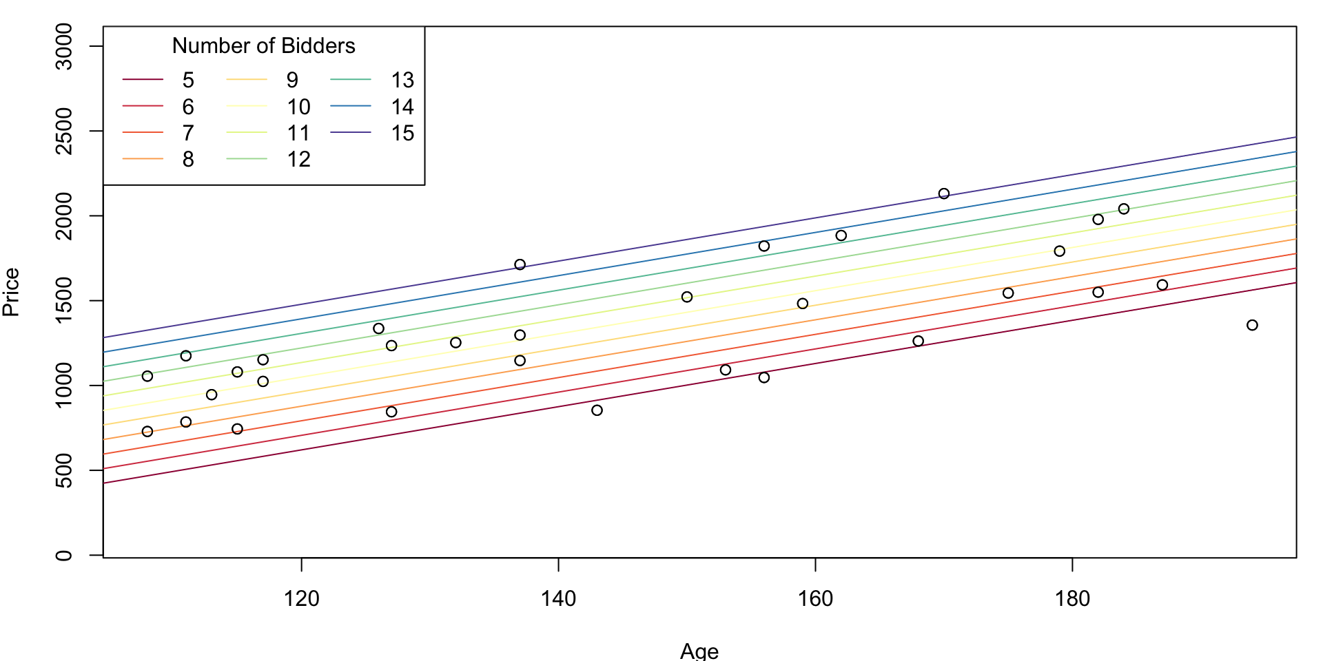
Interaction Model with set Bidders
Show the code
library(RColorBrewer)
par(mar = sm.mar)
plot(Price~Age, ylim = c(100, 3000))
ivec <- seq(from = min(Bidders), to = max(Bidders))
icol <- brewer.pal(n = length(ivec), name = "Spectral")
for (i in 1:length(ivec)){
  abline(a = cf.mod[1] + cf.mod[3]*ivec[i],
         b = cf.mod[2] + cf.mod[4]*ivec[i],
         col = icol[i])
}
points(Age, Price)
legend("topleft", legend = ivec, col = icol, ncol = 3, lty = 1, title = "Number of Bidders")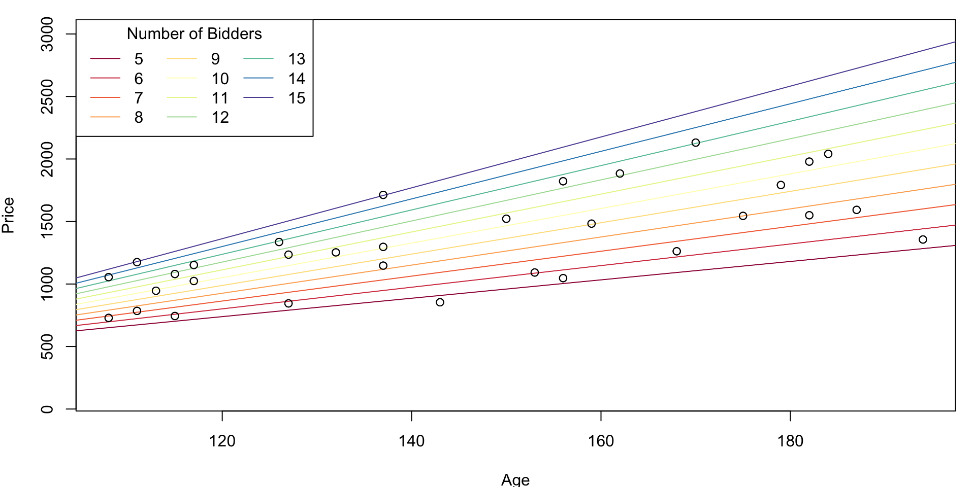
Scatterplot Weight vs Height
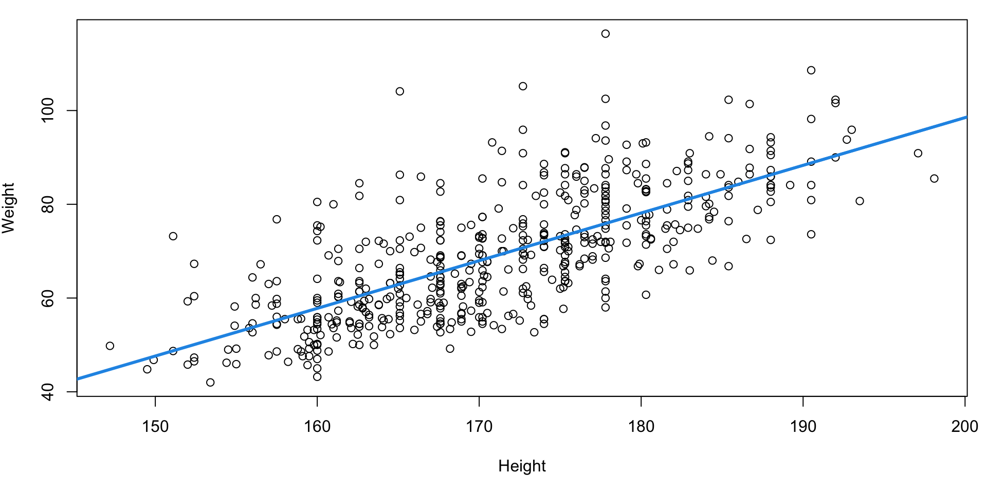
Incorporating Gender
But we know more, eg. gender.
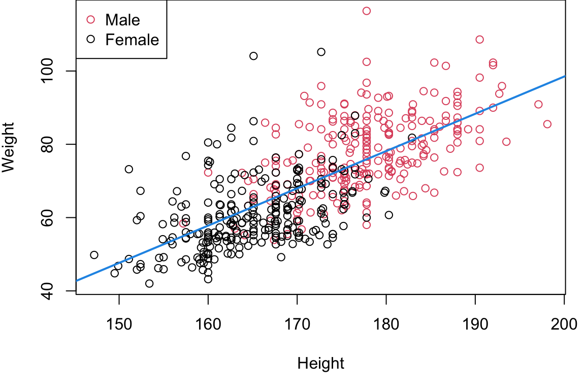
Question: how do we incorporate categorical variables into this model?
Plot of Parallel Slope Model
Show the code
par(mar = c(4, 3.9, 0, 1))        # reduce even more
plot(Weight~Height, col=Gender+1)   # 1 = black, 2 = red (3 = green, 4 = blue ...)
legend("topleft", col=c(2,1), pch=1, legend = c("Male", "Female"))
mcoefs <- mlr$coefficients
abline(mcoefs[1]+ mcoefs[3], mcoefs[2], col=2, lwd=2)
abline(mcoefs[1], mcoefs[2], lwd=2)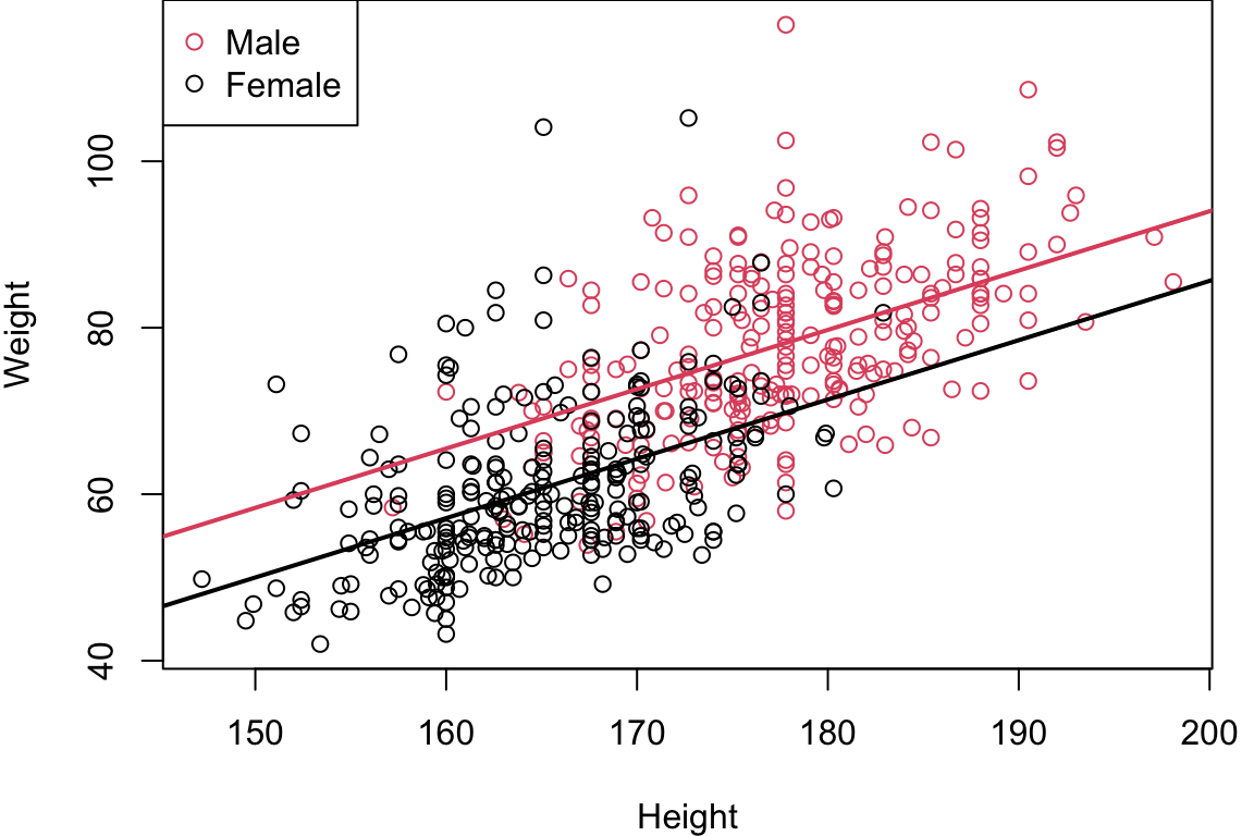
Non-parallel lines
Show the code
# store coeffiecents
icoefs <- intlm$coefficients

# Plot -------
par(mar = c(4.9, 3.9, 1, 1))
plot(Weight~Height, col=Gender+1)
legend("topleft",col=c(2,1),pch=1,
       legend=c("Male","Female"))
# plot the line for males
abline(a = icoefs[1]+ icoefs[3],
       b = icoefs[2] + icoefs[4],
       col=2, lwd=2)
# plot the line for female
abline(a = icoefs[1],
       b= icoefs[2], lwd=2)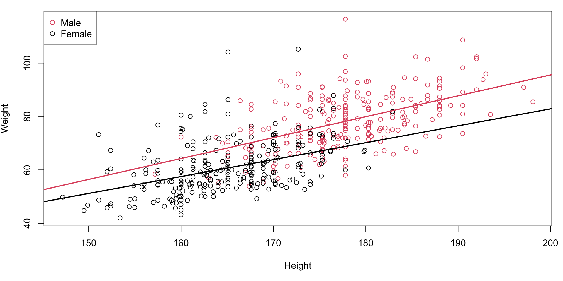
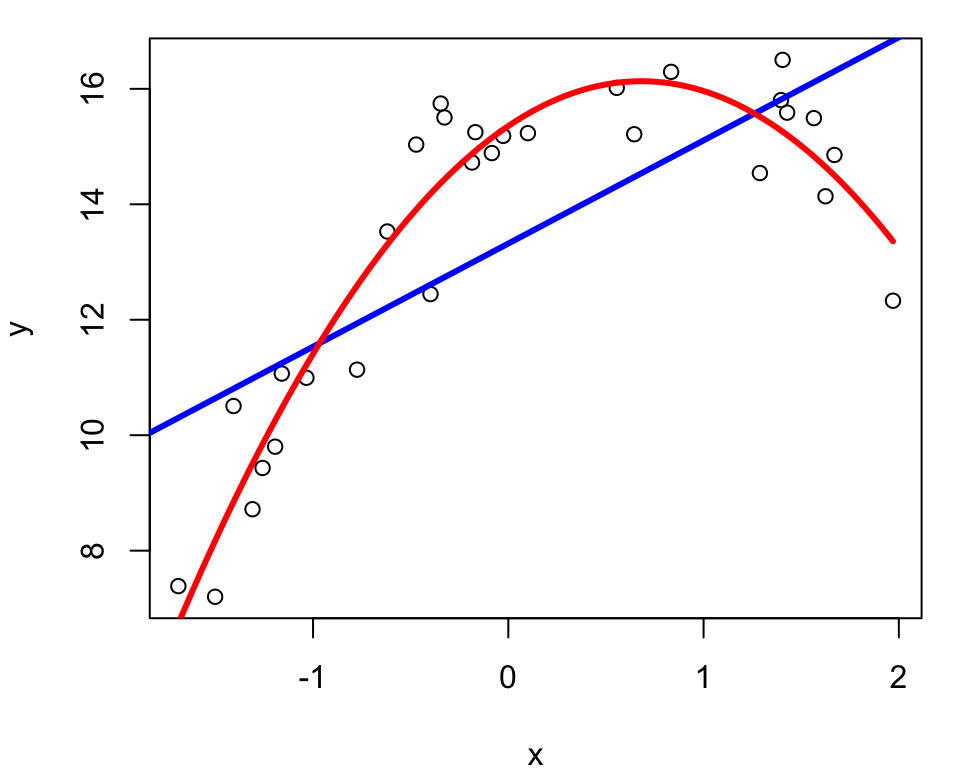
Example: Quadratic Simulation
We simulate 30 values from the following model where \(\epsilon\) is standard normally distributed. \[Y=15+2.3x-1.5x^2+\epsilon\]
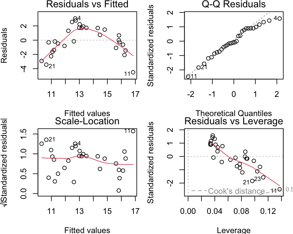
Example: SLR Residuals
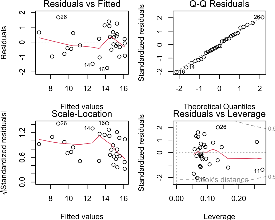
Example: Quadratic Residuals
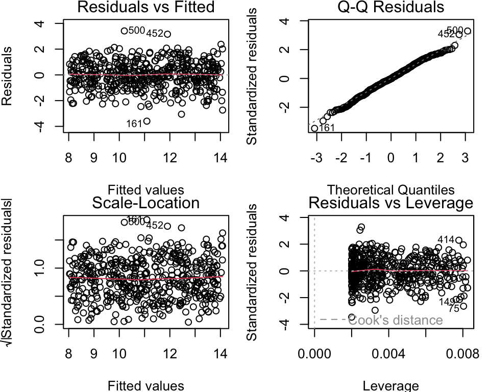
Exemplary Residual Plot
K = 20
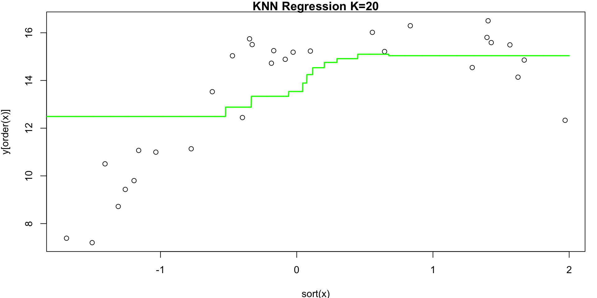
Visualization 1
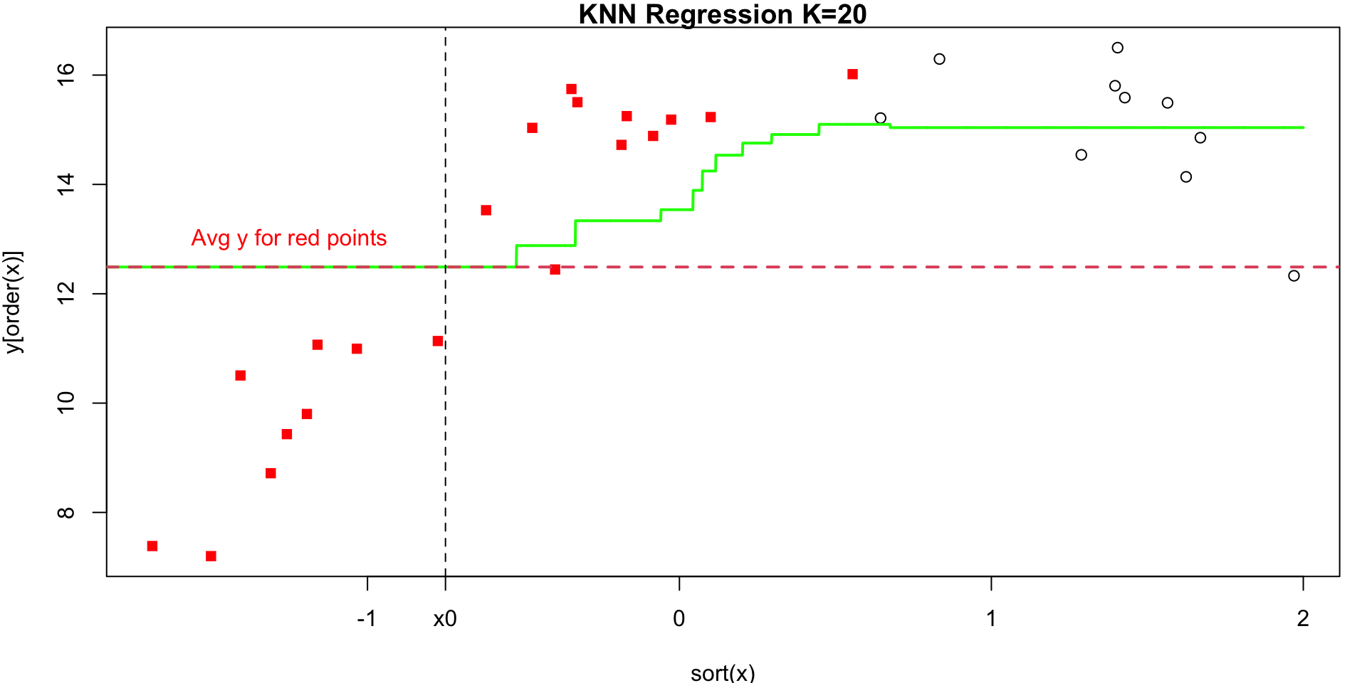
Visualization 2
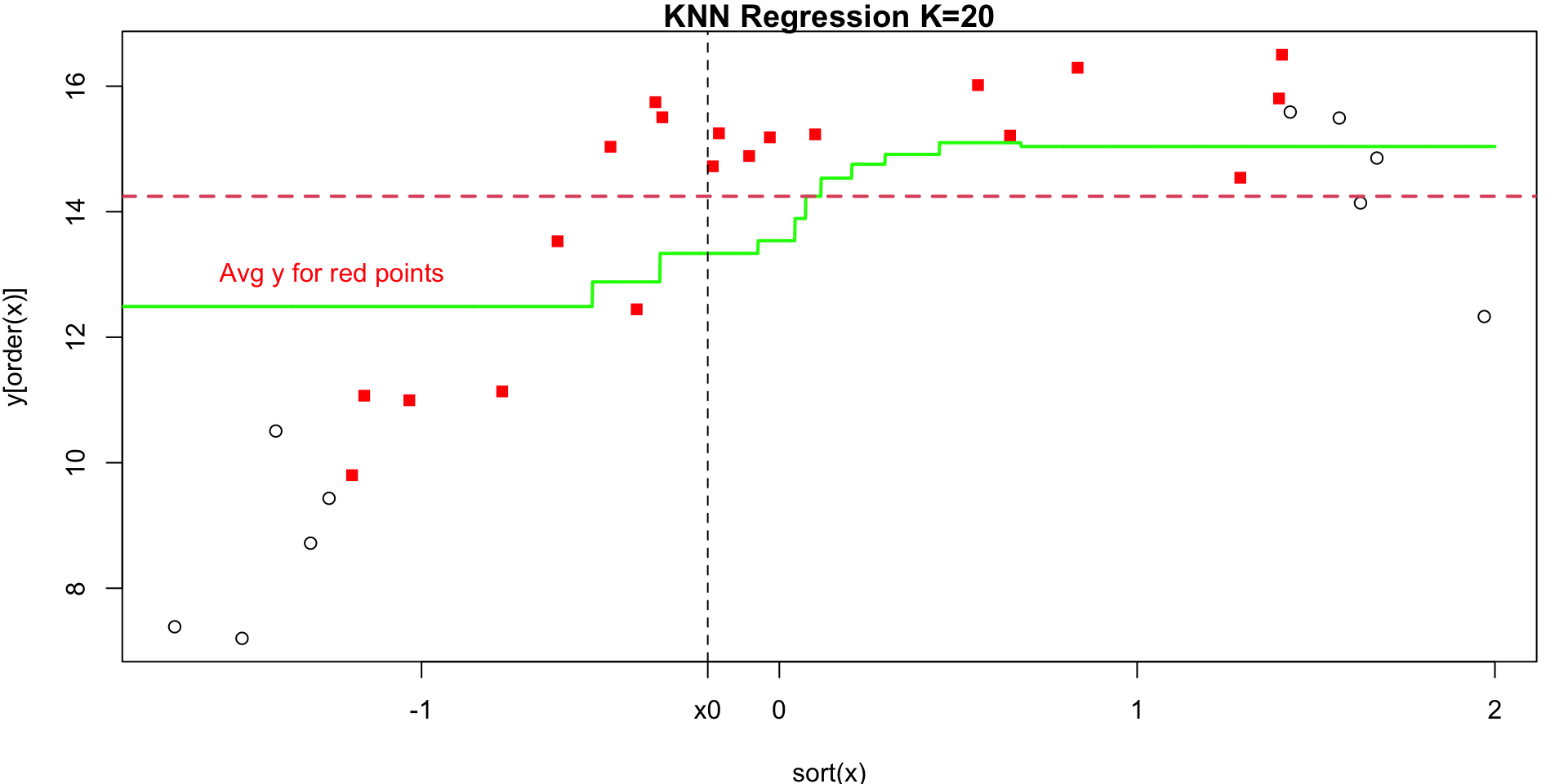
Annimation
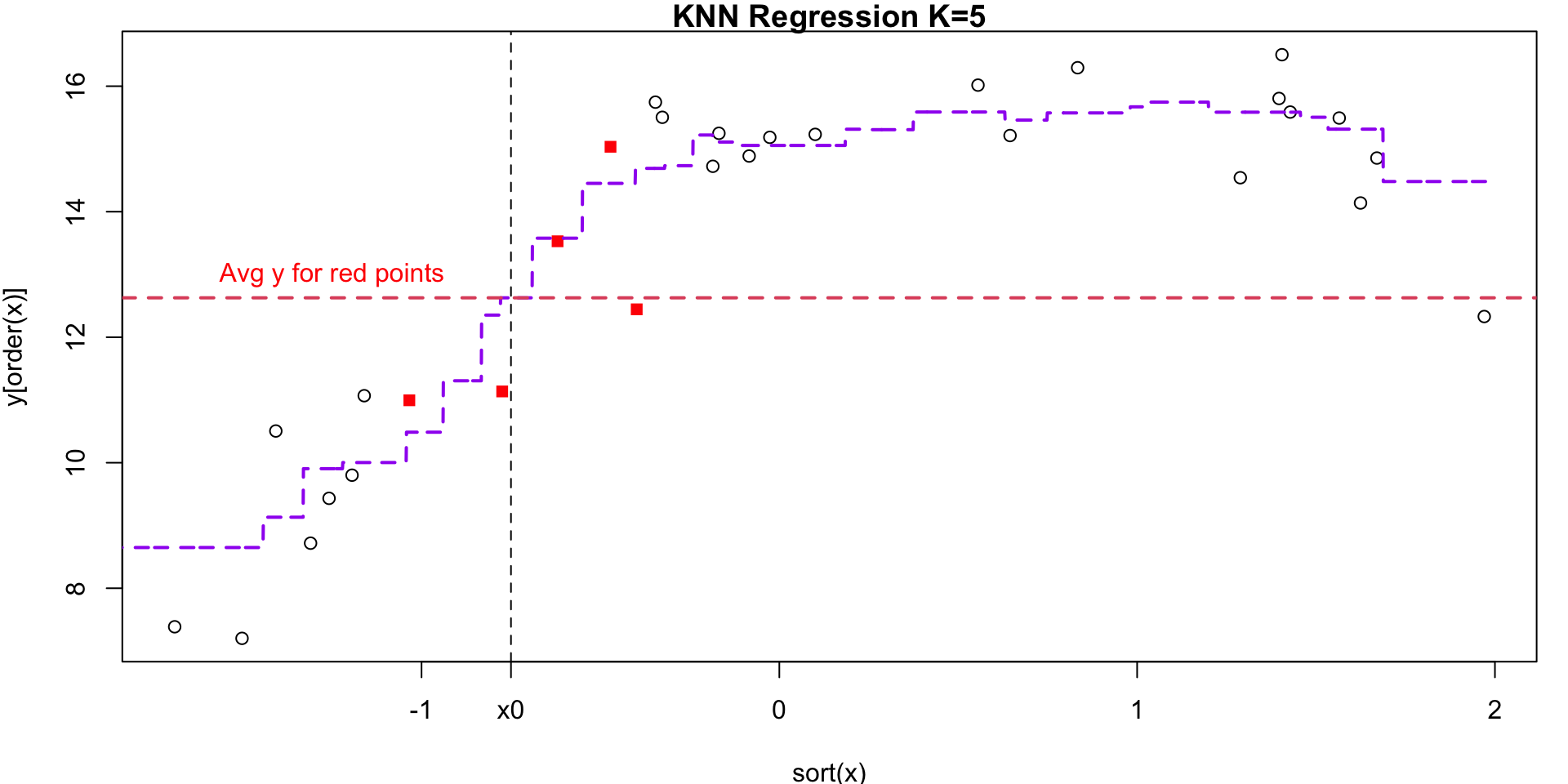
K = 5
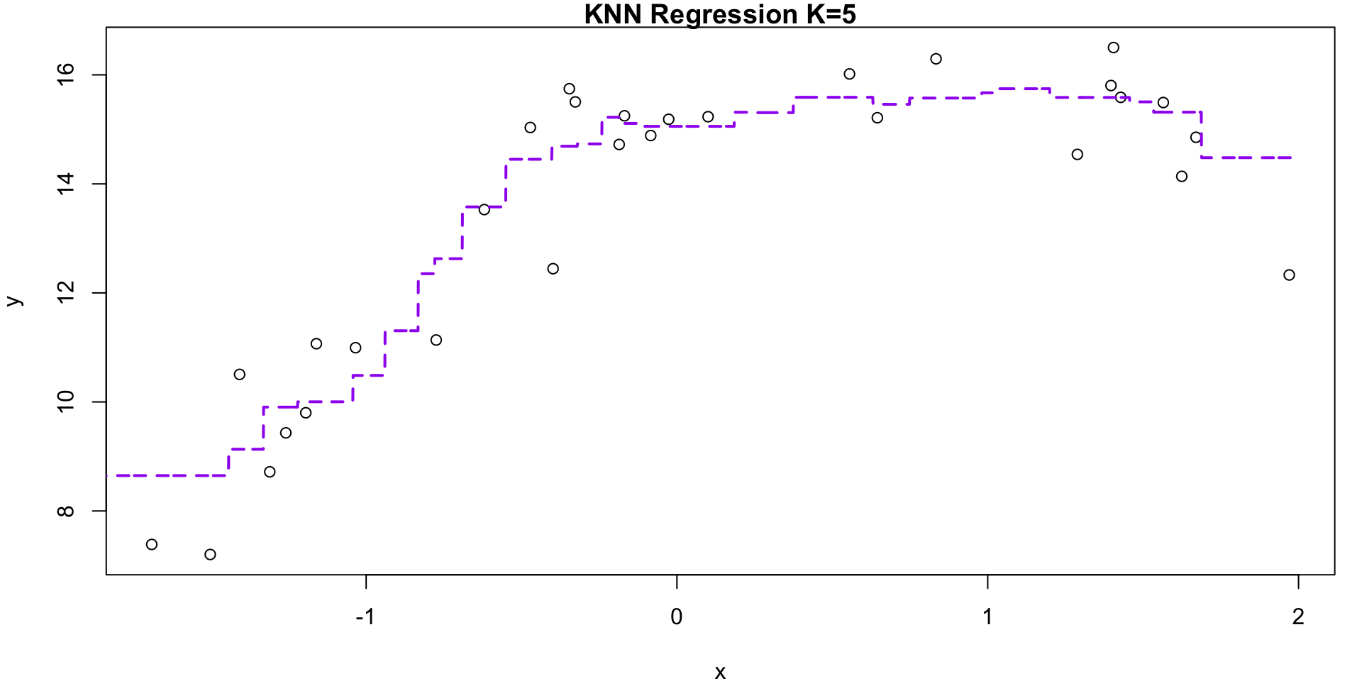
K = 5 Visualization
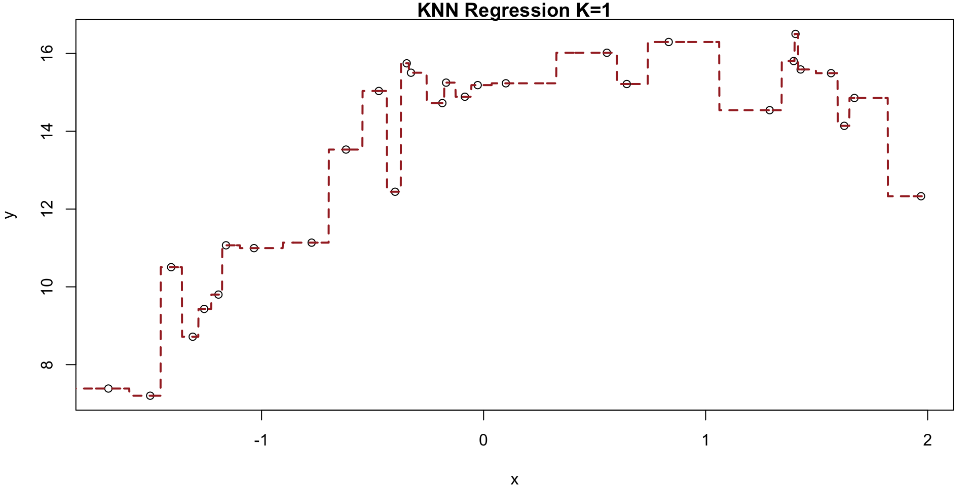
K = 1