Lecture 10: Classification Part 2

DATA 101: Making Prediction with Data

Dr. Irene Vrbik

University of British Columbia Okanagan

Introduction

• Today we continue the introduction to predictive modeling through classification.
• While the previous chapter covered training and data preprocessing, this lecture focuses on how to evaluate the performance of a classifier.
• Unlike last class, today we will do this assessment using the tidymodels framework

Breast Cancer Data

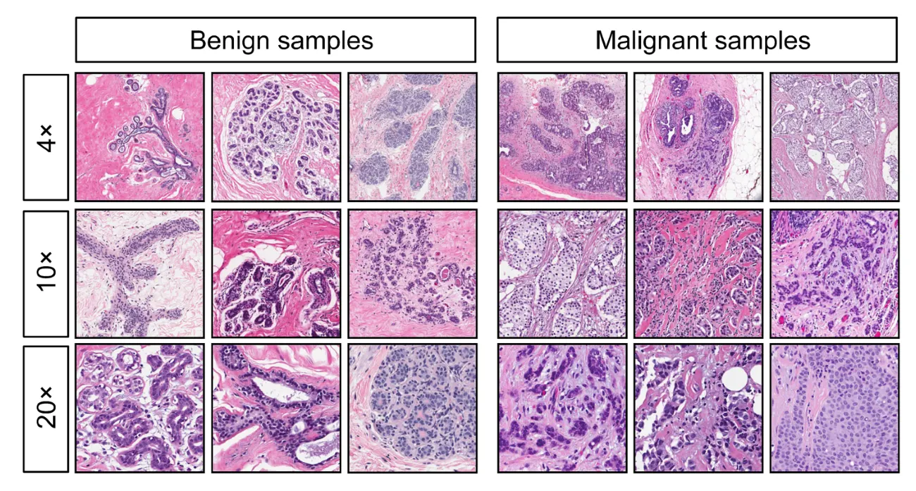
Consider the data set of digitized breast cancer image features, created by Dr. William H. Wolberg, W. Nick Street, and Olvi L. Mangasarian (Street, Wolberg, and Mangasarian 1993).

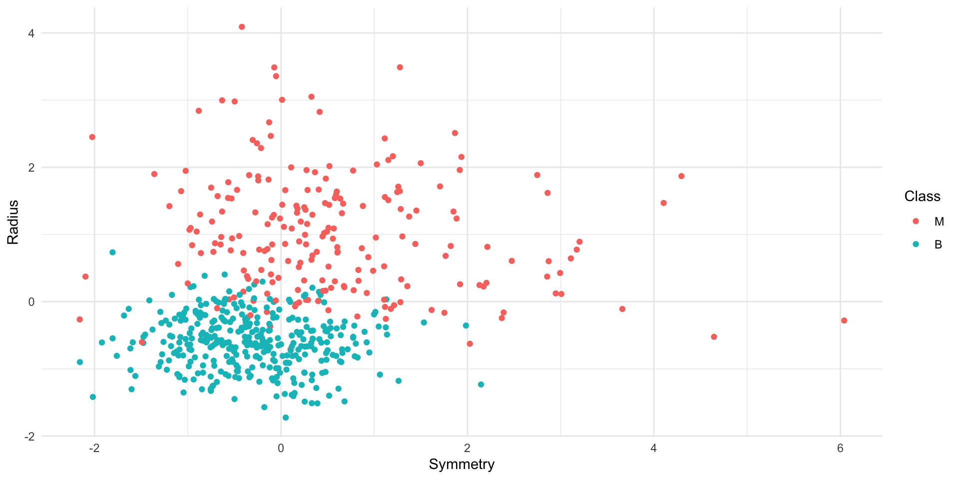
• Each row in the data set represents an image of a tumor sample, including the diagnosis (benign or malignant) and several other measurements (nucleus texture, perimeter, area, and more).
• Diagnosis for each image was conducted by physicians.

Features are computed from a digitized image of a fine needle aspirate (FNA) of a breast mass. They describe characteristics of the cell nuclei present in the image.

Features are computed from a digitized image of a fine needle aspirate (FNA) of a breast mass. They describe characteristics of the cell nuclei present in the image.

Motivation

Task: use these tumor image measurements to predict whether a new tumor image (with unknown diagnosis) shows a benign or malignant tumor.

• Last lectures we talked about how to build a KNN classifier for doing just that.
• Our question we are asking today is:

1. How do we choose \(k\)?
2. How do we evaluate how good this classifier is?

Training error

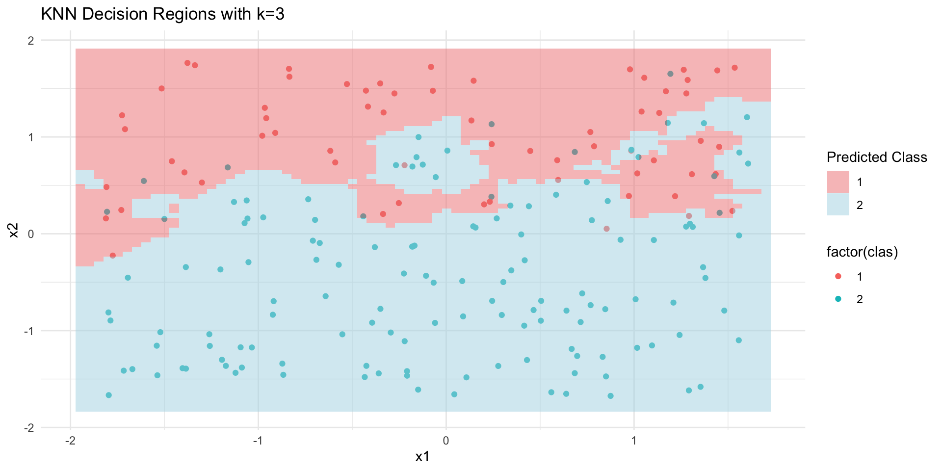
• It is important to realize that sometimes our classifier might make the wrong prediction.
• A classifier does not need to be right 100% of the time to be useful, though we don’t want the classifier to make too many wrong predictions.
• Returning to the example from last class, we see that our KNN classifier would have misclassified some observations in our training set …

Assess Generalization

• But we don’t really care how well our classifier predicts the observations in our training set, but rather if it can be generalized to new observations.

• If our classifier is able to make accurate predictions on data not seen during training it implies that it has actually learned about the relationship between the predictor variables and response variable, as opposed to simply “memorizing” the labels of individual training data.

Testing set

• But what if we don’t have “new” data?

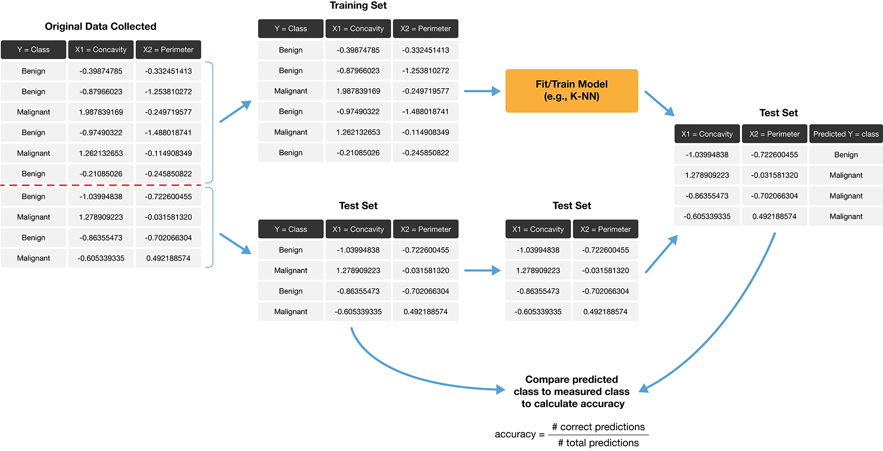
• The trick is to split the data into a training set and testing set

• The training set (only) is used to build our classifier while the testing set is used to evaluate the classifier’s performance.

• If our predictions for the testing set match the true labels, then we have some confidence that our classifier is generalizable and will perform well on new, unseen data.

this last point is crucial for model deployment and real-world applications.

Accuracy

• How exactly can we assess how well our predictions match the true labels for the observations in the test set?

• One way we can do this for classification problems is to calculate the prediction accuracy

• Accuracy is simply the proportion of examples for which the classifier made the correct prediction:

\[\begin{equation} \text{accuracy} = \frac{\text{number of correct predictions}}{\text{total number of predictions}} \end{equation}\]

Deficiency of accuracy

• Accuracy is a convenient, general-purpose way to summarize the performance of a classifier with a single number, but by itself it does not tell the whole story.

• In particular, it does not tell us anything about the kinds of mistakes the classifier makes.

  • e.g. did we mistakenly label a benign tumor malignant
  • or did we mistakenly label a malignant tumor benign

Clearly the second type of mistake is more threatening.

accuracy alone only tells us how often the classifier makes mistakes in general, but ,., (bullet 3)

• A benign tumor is a non-cancerous
• A malignant tumor, commonly referred to as cancer, is a group of abnormal cells that have the potential to invade nearby tissues and spread to other parts of the body, causing harm and potentially life-threatening complications.

Confusion Matrix

• A more comprehensive view of performance can be obtained by additionally examining the confusion matrix.
• A confusion matrix is a tabular representation of a classification model’s performance on a dataset, especially in the context of binary classification.
• The confusion matrix shows how many test set labels of each type are predicted correctly and incorrectly, which gives us more detail about the kinds of mistakes the classifier tends to make.

Example:

	Truly Malignant	Truly Benign
Predicted Malignant	1	4
Predicted Benign	3	57

\[\begin{align} \text{accuracy} &= \frac{\text{number of correct predictions}}{\text{total number of predictions}} \\ &= \frac{1 + 57}{1 + 57 + 4 + 3} = 0.892 \end{align}\]

• 1 malignant observation that was correctly classified as malignant (top left corner),
• 57 benign observations that were correctly classified as benign (bottom right corner).
• it classified 3 malignant observations as benign, and
• 4 benign observations as malignant.

Types of mistakes

• If we just report the single metric, an accuracy of 89% sounds pretty good.
• However, the confusion matrix uncovers that the classifier only identified 1 out of 4 total malignant tumors
• In other words, it misclassified 75% of the malignant cases present in the data set!
• Misclassifying a malignant tumor is a potentially disastrous error, this classifier would likely be unacceptable even with an accuracy of 89%.

• In this example, misclassifying a malignant tumor is a potentially disastrous error, since it may lead to a patient who requires treatment not receiving it.
• Since we are particularly interested in identifying malignant cases, this classifier would likely be unacceptable even with an accuracy of 89%.

General Confusion Matrix

Focusing more on one label than the other is common in classification problems.

	➕	➖
Predicted ➕	✅ TP	❌ FP
Predicted ➖	❌ FN	✅ TN

• When presented with a classification task you should think about which kinds of error are most important.

• Two metrics often reported together with accuracy are precision and recall.

Component of a Confusion matrix

The four main components of a confusion matrix are:

• True Positives (TP): The number of instances correctly predicted as the positive class

• True Negatives (TN): The number of instances correctly predicted as the negative class

• False Positives (FP): The number of instances incorrectly predicted as the positive class

• False Negatives (FN): The number of instances incorrectly predicted as the negative class

• TP: correctly identified as malignant
• TN: correctly identified as benign
• FP: correctly falsely identified as malignant
• FN: correctly falsely identified as benign

Precision

• Precision quantifies how many of the positive predictions the classifier made were actually positive.
• If a classifier has high precision and reports that a new observation is positive, we can trust that the new observation is indeed positive.

\[\begin{equation} \text{precision} = \frac{\text{number of correct positive predictions}}{\text{total number of positive predictions}} \end{equation}\]

• Spam detectors should have high precision We can compute the precision of a classifier using the entries in the confusion matrix, with the formula

Recall

• Recall quantifies how many of the positive observations in the test set were identified as positive.
• When you have a classifier with high recall, it means the classifier is good at finding positive observations and is less likely of missing true positive cases (false negatives are low).

\[\begin{equation} \text{recall} = \frac{\text{number of correct positive predictions}}{\text{total number of positive test set observations}} \end{equation}\]

• Medical Diagnostics should have high recall
• If a classifier with high recall, we can trust that if there is a positive observation in the test data, it will find it.

Example (cont’d)

Returning to this example, we have the following calculations for precision and recall:

\[\begin{align} \text{precision} &= \frac{1}{1 + 4} = 0.20\\ \text{recall} &= \frac{1}{1 + 3} = 0.25. \end{align}\]

So even with an accuracy of 89%, the precision and recall of the classifier were both relatively low.

Comment

• It is difficult to achieve both high precision and high recall at the same time
• Models with high precision tend to have low recall
  1. we can make a classifier that has perfect recall: just always guess positive! however, this will make lots of false positive (low precision)
• Models with high recall tend to have low precision
  2. we can make a classifier that has perfect precision: never guess positive! however, this will make lots of false negative (0% recall!)

Of course, most real classifiers fall somewhere in between these two extremes.

• This classifier will of course find every positive observation in the test set, but it will make lots of false positive predictions along the way and have low precision.
• there is a trade-off between precision and recall that one has to make when designing a classifier.
• But these examples serve to show that in settings where one of the classes is of interest (i.e., there is a positive label),

Training/Testing splits

• Unlike the visualization suggests, we do not simply take the first, say 60% of observations to be our training set, and the remaining 40% to be the test.

• For one reason, data often come ordered in some way (e.g. by date) so we would not like to add that bias to our training set.

• Rather than manually selecting observation, what we will do is split the data set randomly into training and test set.

this avoid accidentally influencing the result of the evaluation.

The training-testing split is not fixed and can vary depending on the specific problem, dataset size, and objectives; 50/50, 70/30 and 80/20 are also quite common.

Randomness and seeds

• We use randomness any time we need to make a decision in our analysis that needs to be fair, unbiased, and not influenced by human input.
• However, the use of randomness runs counter to one of the main tenets of good data analysis practice: reproducibility¹
• The trick is that in R—and other programming languages—randomness is not actually random!

• Our data analyses will often involve the use of randomness.
• if we include randomness in the analysis, would we not get a different result each time?

1. Recall that a reproducible analysis produces the same result each time it is run

Pseudorandom

• Pseudorandom, or pseudo-random, refers to a sequence of numbers or values that appears to be random but is generated by a deterministic process, typically a mathematical algorithm.

• In other words, pseudorandom sequences are not truly random but are instead generated in a way that simulates randomness.

• R’s random number generator produces a sequence of numbers that are completely determined by a seed value.

• making them suitable for various applications where true randomness is not required or feasible

set.seed

In the R programming language, the set.seed() function is used to set the seed for the random number generator.

# random numbers without a seed
# sample 1
sample(0:9, 10, replace=TRUE)

 [1] 5 0 8 0 0 6 7 9 0 2

# sample 2
sample(0:9, 10, replace=TRUE)

 [1] 8 4 5 9 0 5 8 0 2 5

# sample 3
sample(0:9, 10, replace=TRUE)

 [1] 4 6 9 6 1 6 5 2 0 6

# random numbers with a seed
set.seed(2023)
sample(0:9, 10, replace=TRUE)

 [1] 4 8 7 2 9 1 0 0 0 0

set.seed(2023)
sample(0:9, 10, replace=TRUE)

 [1] 4 8 7 2 9 1 0 0 0 0

set.seed(2023)
sample(0:9, 10, replace=TRUE)

 [1] 4 8 7 2 9 1 0 0 0 0

• This is not specific to my computer. If you copy and paste the code with a seed in your R session you will get the same thing too
• without the seed you’ll get something diffent every time

Even though the sequences of numbers that R is generating look random, they are totally determined when we set a seed value!

Comment

• Many functions in tidymodels, tidyverse use randomness¹

• At the beginning of every data analysis you do, right after loading packages, you should call the set.seed() function and pass it an integer of your choosing.

• If you do not explicitly “set a seed” your results will likely not be reproducible.

• Avoid setting a seed many times throughout your analysis, otherwise the randomness that R uses will not look as random as it should.

• sample is certainly not the only function that uses randomness in R.
• be careful to set the seed only once at the beginning of a data analysis. If you use
• Each time you set the seed, you are inserting your own human input, thereby influencing the analysis.
• Also note that when R starts up, it creates its own seed to use.

1. for example, KNN flips a coin when there is a tie in the majority voting

Swith it up!

• In my notes you might find that I often use the year as my random seed …
• Using the same seed repeated could lead to a using the same seed fixed sequence of pseudorandom numbers.
• For this reason, it would recommend using a variety of seeds

tidymodels

• Tidymodels is a collection of R packages and tools for modeling and machine learning that follow the principles of tidy data science

• It powerful and flexible framework for conducting end-to-end machine learning and predictive modeling in R while promoting best practices for data science and analysis.

• We can use the tidymodels package not only to perform KNN classification, but also to assess how well our classification worked.

Example: Breast Cancer

• Let’s work through an example of how to use tools from tidymodels to evaluate a classifier using the breast cancer data set; csv can be downloaded here.

• In line with our previous discussion, let’s load our required packages and set a seed to begin:

# load packages
library(tidyverse)
library(tidymodels)

# set the seed
set.seed(1)

Load and visualize

# load data
cancer <- read_csv("data/wdbc_unscaled.csv") |>
  # convert the character Class variable to the factor datatype
  mutate(Class = as_factor(Class))  |>
  # rename the factor values to be more readable
  mutate(Class = fct_recode(Class, "Malignant" = "M", "Benign" = "B"))

# create scatter plot of tumor cell concavity versus smoothness,
# labeling the points be diagnosis class
perim_concav <- cancer |>
  ggplot(aes(x = Smoothness, y = Concavity, color = Class)) +
  geom_point(alpha = 0.5) +
  labs(color = "Diagnosis") +
  scale_color_manual(values = c("orange2", "steelblue2")) + 
  theme(text = element_text(size = 12))

perim_concav

Load and visualize

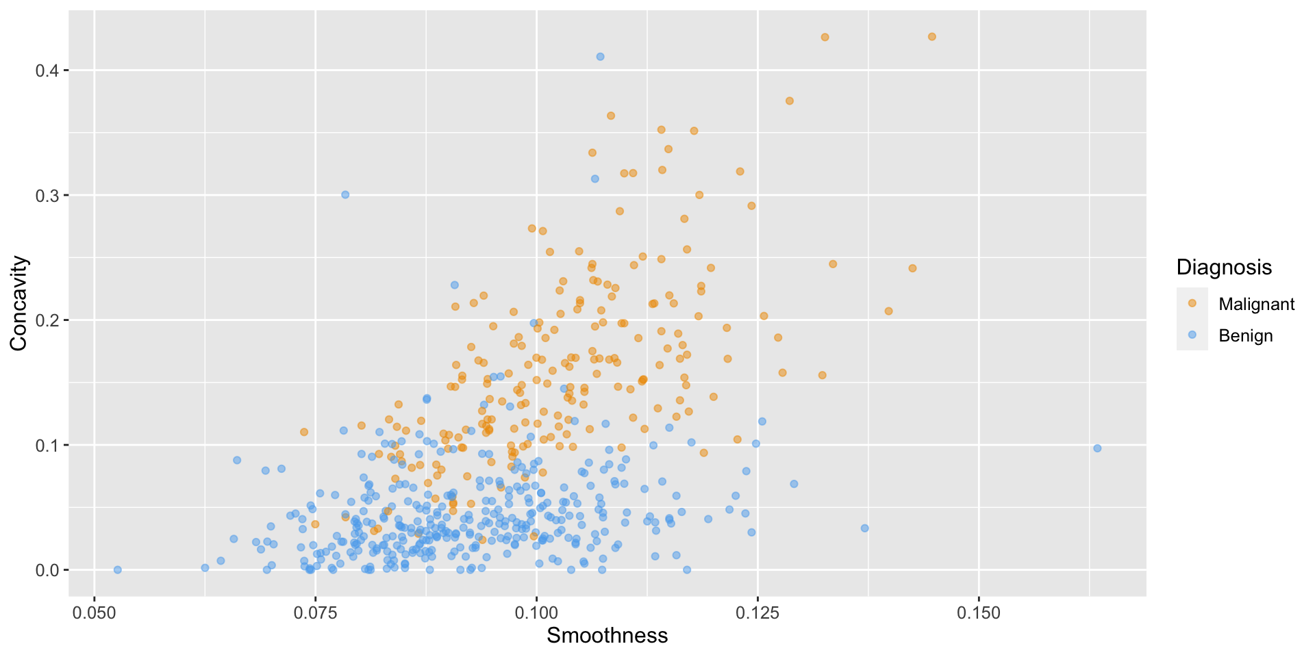
Create the train / test split

• Typically, the training set is between 50% and 95% of the data, while the test set is the remaining 5% to 50%
• The intuition is that you want to trade off between training an accurate model (by using a larger training data set) and getting an accurate evaluation of its performance (by using a larger test data set).
• Here, we will use 75% of the data for training, and 25% for testing.

initial_split

The initial_split() function from tidymodels splits the data while applying two very important steps:

1. it shuffles the data before splitting
2. it stratifies the data by the class label, to ensure that roughly the same proportion of each class ends up in both the training and testing sets.

Example: if our data comprise roughly 63% benign observations, and 37% malignant, initial_split ensures that roughly 63% of the training data are benign, 37% of the training data are malignant, and the same proportions exist in the testing data.

These steps help to ensure that the accuracy estimates from the test data are reasonable.

1. ensures that any ordering present in the data does not influence the data that ends up in the training and testing sets.

?initial_split

initial_split(data, prop = 3/4, strata = NULL)

• data A data frame.
• prop The proportion of data to be retained for modeling/analysis.
• strata A variable in data (single character or name) used to conduct stratified sampling. When not NULL, each resample is created within the stratification variable¹

1. Numeric strata are binned into quartiles.

initial_split for splitting

cancer_split <- initial_split(cancer, prop = 0.75, strata = Class)

• specify that prop = 0.75 so that 75% of our original data set ends up in the training set (and the remaining 25% makes up our testing set)

• set the strata argument to the categorical label variable (here, Class) to ensure that the training and testing subsets contain the right proportions of each category of observation.

R: Training and Testing sets

cancer_train <- training(cancer_split)
cancer_test <- testing(cancer_split) 

glimpse(cancer_train)

Rows: 426
Columns: 12
$ ID                <dbl> 8510426, 8510653, 8510824, 857373, 857810, 858477, 8…
$ Class             <fct> Benign, Benign, Benign, Benign, Benign, Benign, Beni…
$ Radius            <dbl> 13.540, 13.080, 9.504, 13.640, 13.050, 8.618, 10.170…
$ Texture           <dbl> 14.36, 15.71, 12.44, 16.34, 19.31, 11.79, 14.88, 20.…
$ Perimeter         <dbl> 87.46, 85.63, 60.34, 87.21, 82.61, 54.34, 64.55, 54.…
$ Area              <dbl> 566.3, 520.0, 273.9, 571.8, 527.2, 224.5, 311.9, 221…
$ Smoothness        <dbl> 0.09779, 0.10750, 0.10240, 0.07685, 0.08060, 0.09752…
$ Compactness       <dbl> 0.08129, 0.12700, 0.06492, 0.06059, 0.03789, 0.05272…
$ Concavity         <dbl> 0.066640, 0.045680, 0.029560, 0.018570, 0.000692, 0.…
$ Concave_points    <dbl> 0.047810, 0.031100, 0.020760, 0.017230, 0.004167, 0.…
$ Symmetry          <dbl> 0.1885, 0.1967, 0.1815, 0.1353, 0.1819, 0.1683, 0.27…
$ Fractal_dimension <dbl> 0.05766, 0.06811, 0.06905, 0.05953, 0.05501, 0.07187…

nrow(cancer_train)/nrow(cancer)

[1] 0.7486819

cancer_proportions <- cancer_train |>
                      group_by(Class) |>
                      summarize(n = n()) |>
                      mutate(percent = 100*n/nrow(cancer_train))

cancer_proportions

glimpse(cancer_test)

Rows: 143
Columns: 12
$ ID                <dbl> 84501001, 846381, 84799002, 849014, 852763, 853401, …
$ Class             <fct> Malignant, Malignant, Malignant, Malignant, Malignan…
$ Radius            <dbl> 12.460, 15.850, 14.540, 19.810, 14.580, 18.630, 16.7…
$ Texture           <dbl> 24.04, 23.95, 27.54, 22.15, 21.53, 25.11, 21.59, 18.…
$ Perimeter         <dbl> 83.97, 103.70, 96.73, 130.00, 97.41, 124.80, 110.10,…
$ Area              <dbl> 475.9, 782.7, 658.8, 1260.0, 644.8, 1088.0, 869.5, 5…
$ Smoothness        <dbl> 0.11860, 0.08401, 0.11390, 0.09831, 0.10540, 0.10640…
$ Compactness       <dbl> 0.23960, 0.10020, 0.15950, 0.10270, 0.18680, 0.18870…
$ Concavity         <dbl> 0.22730, 0.09938, 0.16390, 0.14790, 0.14250, 0.23190…
$ Concave_points    <dbl> 0.085430, 0.053640, 0.073640, 0.094980, 0.087830, 0.…
$ Symmetry          <dbl> 0.2030, 0.1847, 0.2303, 0.1582, 0.2252, 0.2183, 0.18…
$ Fractal_dimension <dbl> 0.08243, 0.05338, 0.07077, 0.05395, 0.06924, 0.06197…

nrow(cancer_test)/nrow(cancer)

[1] 0.2513181

table(cancer_test$Class)/nrow(cancer_test)

Malignant    Benign 
0.3706294 0.6293706 

• Let’s use the initial_split function to create the training and testing sets.

• The training and testing functions then extract the training and testing data sets into two separate data frames. Note that the initial_split function uses randomness, but since we set the seed earlier in the chapter, the split will be reproducible.

Data Preprocessing

• In the tidymodels framework, all data preprocessing happens using a recipe from the recipespackage.
• Here we will initialize a recipe for the cancer_train data, specifying that:
  • Class is the response, and Smoothness and Concavity are to be used as predictors.

?recipe

A recipe is a description of the steps to be applied to a data set in order to prepare it for data analysis.

recipe(x, ...)

x, data	A data frame or tibble of the template data set (see below).
...	Further arguments passed to or from other methods (not currently used).
formula	A model formula of the form y~x1+x2+ ... + xp where y is your response variable and x1, x2, …, xp are your desired predictors

As discussed last class, KNN is sensitive to the scale of the predictor, hence, we standardize them…

To use all remaining columns of your dataset as predictors, use the shortcut y~.

recipe for normalizing

cancer_recipe <- recipe(Class ~ Smoothness + Concavity, 
                        data = cancer_train) |>
                step_scale(all_predictors()) |>
                step_center(all_predictors())

• step_scale creates a scaling step that will normalize numeric data to have a standard deviation of one.
• step_center creates a centering step that will normalize numeric data to have a mean of zero
• all_predictors() is used to select variables

Alternatives include: all_numeric_predictors, all_nominal_predictors, all_factor

Comment

• step_normalize both centering and scaling in a single recipe step; however we will keep step_scale and step_center separate to emphasize conceptually that there are two steps happening

• Notice how we are only doing this standardization over the training set.
• This avoids “peaking” at our test set and ensures that our test data does not influence any aspect of our model training.

An additional consideration we need to take when doing this is that we should create the standardization preprocessor using only the training data. This ensures that our test data does not influence any aspect of our model training. Once we have created the standardization preprocessor, we can then apply it separately to both the training and test data sets.

Training the classifer

• Now that we have split our original data set into training and test sets, we can create our KNN classifier with only the training set.

• For now, we will just choose the number \(k\), the number of nearest neighbors, to be 3

• We use Concavity and Smoothness as the predictors (as specified in our recipe)

• While we did this with the knn function from the class package last class, let’s see how we can do it with the tidymodels functions …

Model specification

knn_spec <- nearest_neighbor(neighbors = 3)

• First, we need create a model specification for KNN classification by calling the nearest_neighbor function, specifying that we want to use K=3 neighbors

Model specification

knn_spec <- nearest_neighbor(weight_func= , neighbors = 3)

• The weight_func argument controls how neighbors vote when classifying a new observation

Model specification

knn_spec <- nearest_neighbor(weight_func="rectangular", neighbors = 3)

• The weight_func argument controls how neighbors vote when classifying a new observation

• weight_func = "rectangular" specifies that each neighboring point should have the same weight when voting

• Other choices, which weigh each neighbor’s vote differently, can be found on the parsnip website.

Model specification

knn_spec <- nearest_neighbor(weight_func="rectangular", neighbors = 3) |>
  set_engine("kknn")

• In the set_engine argument, we specify which package or system will be used for training the model.
• Here kknn is the R package we will use for performing KNN classification.

Model specification

knn_spec <- nearest_neighbor(weight_func="rectangular", neighbors = 3) |>
  set_engine("kknn") |>
  set_mode("classification")

• In the set_engine argument, we specify which package or system will be used for training the model.
• Here kknn is the R package we will use for performing KNN classification.
• Finally, we specify that this is a classification problem with the set_mode function.

Fitting the model

• In order to fit the model on the breast cancer data, we need to pass the model specification and the data set to the fit function.

• While we could use something like the following, this would not include the data preprocessing steps

• In order to include our “recipe” from before, we need to adopt a tidymodels workflow

workflow

• The tidymodels package collection also provides the workflow, a way to chain together multiple data analysis steps without a lot of otherwise necessary code for intermediate steps.

• This framework combines data preprocessing steps, model specification, and model fitting into a single cohesive unit.

• Workflows help you streamline and simplify the process of building, tuning, and evaluating predictive models while following the principles of tidy data science.

workflow example

knn_fit <- workflow() |>
  add_recipe(cancer_recipe) |>
  add_model(knn_spec) |>
  fit(data = cancer_train)

knn_fit

══ Workflow [trained] ══════════════════════════════════════════════════════════
Preprocessor: Recipe
Model: nearest_neighbor()

── Preprocessor ────────────────────────────────────────────────────────────────
2 Recipe Steps

• step_scale()
• step_center()

── Model ───────────────────────────────────────────────────────────────────────

Call:
kknn::train.kknn(formula = ..y ~ ., data = data, ks = min_rows(3,     data, 5), kernel = ~"rectangular")

Type of response variable: nominal
Minimal misclassification: 0.1150235
Best kernel: rectangular
Best k: 3

Prediction

• Now that we have a KNN classifier object, we can use it to predict the class labels for our test set.

• We use the bind_cols to add the column of predictions to the original test data, creating the cancer_test_predictions data frame.

• The Class variable contains the true diagnoses, while the .pred_class contains the predicted diagnoses from the classifier.

cancer_test_predictions <- predict(knn_fit, cancer_test) |>
  bind_cols(cancer_test)

cancer_test_predictions

Prediction

Evaluate performance

• Finally, we can assess our classifier’s performance; first let’s examine accuracy.
• To do this we use the metrics function from tidymodels, specifying the truth and estimate arguments:

cancer_test_predictions |>
  metrics(truth = Class, estimate = .pred_class) |>
  filter(.metric == "accuracy")

.metric

• In the metrics data frame, we filtered the .metric column since we are interested in the accuracy row.
• Other entries involve other metrics that are beyond the scope of this course.
• Looking at the value of the .estimate variable shows that the estimated accuracy of the classifier on the test data was 86%.

conf_mat

• We can also look at the confusion matrix for the classifier, which shows the table of predicted labels and correct labels, using the conf_mat function:

confusion <- cancer_test_predictions |>
             conf_mat(truth = Class, estimate = .pred_class)
confusion

           Truth
Prediction  Malignant Benign
  Malignant        39      6
  Benign           14     84

• 39 observations were correctly predicted as malignant, and
• 84 were correctly predicted as benign.

mistakes; in particular,

• it classified 14 observations as benign when they were truly malignant, and
• 6 observations as malignant when they were truly benign.

Other metrics

Using our formulas from earlier, we see that the accuracy agrees with what R reported, and can also compute the precision and recall of the classifier:

\[\begin{align} \mathrm{accuracy} &= \frac{\mathrm{number \; of \; correct \; predictions}}{\mathrm{total \; number \; of \; predictions}} = \frac{39+84}{39+84+6+14} = 0.86\\ \mathrm{precision} &= \frac{\mathrm{number \; of \; correct \; positive \; predictions}}{\mathrm{total \; number \; of \; positive \; predictions}} = \frac{39}{39 + 6} = 0.867\\ \mathrm{recall} &= \frac{\mathrm{number \; of \; correct \; positive \; predictions}}{\mathrm{total \; number \; of \; positive \; test \; set \; observations}} = \frac{39}{39+14} = 0.736 \end{align}\]

Final comments

• In this example we have somewhat arbitrarily set the number of nearest neighbours to \(k\)
• Next class we will see how we can use cross-validation to choose this value for us